Modern Economy, 2012, 3, 584-589
http://dx.doi.org/10.4236/me.2012.35077 Published Online September 2012 (http://www.SciRP.org/journal/me)
Relationship between Trading Volume and Asymmetric
Volatility in the Korean Stock Market
Ki-Hong Choi1, Zhu-Hua Jiang2, Sang Hoon Kang3, Seong-Min Yoon1*
1Department of Economics, Pusan National University, Busan, Korea
2Research Institute of Social Criticality, Pusan National University, Busan, Korea
3Department of Business Administration, Pusan National University, Busan, Korea
Received May 27, 2012; revised June 25, 2012; accepted July 5, 2012
ABSTRACT
We investigated the relationship between return volatility and trading volume as a proxy for the arrival of information
to the market, based on Korean stock market (KSM) data from January 2000 to December 2010. We measured the rela-
tionship between return volatility and trading volume using the GJR-GARCH and exponential GARCH (EGARCH)
models. We found a positive relationship between trading volume and volatility, suggesting that trading volume influ-
ences the flow of information to the market. This finding supports the validity of the mixture of distributions hypothesis.
Considering that trading volume can also explain volatility asymmetry, we conclude that trading volume is a useful tool
for predicting the volatility dynamics of the KSM.
Keywords: Asymmetry; Volatility; Trading Volume; Mixture of Distribution Hypothesis
1. Introduction
Volatility exhibits three typical patterns in most financial
time series, namely, clustering, asymmetry, and persistence.
In particular, many empirical studies have identified asym-
metric volatility, by which stock return volatility tends to
rise more following a large fall in price (bad news) than
following a rise in price (good news) (Nelson [1]; Engle
and Ng [2]). We investigated the effects of trading volume
on asymmetric volatility in the Korean stock market (KSM),
by studying the relationship between volatility and trading
volume as a proxy for the arrival of information (herea-
fter, information arrival) to the market.
We examined the relationship between stock returns
and trading volume using the mixture of distributions
hypothesis (MDH), in the context of information arrival.
The MDH provides an explanation for volatility and
volume by linking changes in price, volume, and the rate
of information flow. The MDH implies a positive relat-
ionship between trading volume and volatility, as price
changes simultaneously. Shifts to new equilibrium are
immediate, and no intermediate processes form.
Many empirical studies supporting the MDH have exp-
lained volatility persistence by including trading volume
as a proxy for information arrival using the general auto-
regressive conditional heteroskedasticity (GARCH) model.
But almost none of these studies considered asymmetric
GARCH models. This study used the daily stock index
and its trading volume on the KSM to explore the rela-
tionship between asymmetric volatility and trading volu-
me, using two asymmetric GARCH models; exponential
GARCH (EGARCH) and Glosten-Jagannathan-Runkle-
GARCH (GJR-GARCH) models.
The remainder of this paper is organized as follows. A
literature review is presented in Section 2. Section 3 pre-
sents the data and descriptive statistics. Section 4 presents
the methodology of the study. The empirical results are
discussed in Section 5. Section 6 concludes the paper.
2. Literature Review
Economists have long been interested in studying the
relationship between stock return volatility and trading
volume. Studies on this relationship are usually theoreti-
cally based on either the sequential information arrival
hypothesis (SIAH) or the MDH.
The seminal study of Copeland [3] assumed that traders
receive new information in sequential random style; acco-
rdingly, he developed the SIAH. The traders change their
trading positions as new information arrives to the market.
However, not all traders receive this new information at
exactly the same time. Hence, the response of each indi-
vidual trader to this information represents an incomplete
equilibrium. The final market equilibrium is established
when all traders have received the information and have
made a trading decision based on that information. Thus,
*Corresponding author.
C
opyright © 2012 SciRes. ME

K.-H. CHOI ET AL. 585
the SIAH suggests that a lead-lag relationship between
volume and volatility exists only in the presence of inf-
ormation.
However, the MDH offers a different explanation by
linking changes in price, volume, and rate of information
flow (Clark [4]; Epps and Epps [5]; Harris [6]). The MDH
implies a positive relationship between trading volume
and price variability, and this relationship is a function of
a mixing variable defined as the rate of information flow.
In the MDH, the shift to a new equilibrium is immediate,
and the partial equilibrium of the sequential information
model never occurs. Clark [4] introduced this concept,
which explores the role of trading volume as a proxy for
a stochastic process of information arrival, for theoretically
analyzing trading volume and the movement of stock
prices.
Lamoureux and Lastrapes [7], testing the relationship
between volume and volatility for a number of actively
traded stocks in the United States, used contemporaneous
trading volume as an explanatory variable in the variance
equation and found that the inclusion of volume eliminated
the persistence of volatility. Gallo and Pacini [8], using
data on 10 actively traded US stocks from 1985 to 1995,
found that persistence decreased when trading volume
was used in the conditional variance equation. Foster [9]
tested the predictions of MDH for the oil futures market
from 1990 to 1994 and found that volume and volatility
were largely contemporaneously related and that both
were driven by the same factor, which is assumed to be
information arrival. Alsubaie and Najand [10] tested the
effect of trading volume on the persistence of the con-
ditional volatility of returns in the Saudi stock market.
Overall, their results supported the MDH at the firm level.
However, not all studies support the MDH. For example,
Sharma, Mbodja and Kamath [11] investigated the relati-
onship between trading volume and volatility for the New
York Stock Exchange (NYSE) index from 1986 to 1989.
They found that trading volume did not completely explain
the GARCH effect, and concluded that while trading
volume might be a good proxy for information arrival
about individual firms, it is not true for the market as a
whole. Lee [12] investigated the relationship between
trading volume and volatility of Korean markets using
the threshold GARCH (TGARCH) model and found that
there was asymmetric volatility in the Korea Composite
Stock Price Index (KOSPI) and the Korean Securities
Dealers Automated Quotations (KOSDAQ) market, but
concluded that inclusion of trading volume did not reduce
volatility persistence in the conditional variance equation.
An, Jang and Lee [13] examined the contemporaneous
correlation as well as the lead-lag relationship between
trading volume and return volatility on the Korean stock
market and found evidence of a significant lead-lag rela-
tionship between trading volume and the return volatility
using the SIAH. Kim and Kim [14] investigated the rela-
tionship between return volatility and volume of the KOSPI
200 futures index using the GJR-GARCH model. They
identified volatility persistence, asymmetric responses to
information arrival, and a relationship between return
volatility and volume.
3. Data and Descriptive Statistics
Our primary data set consisted of a daily stock index and
its trading volume on the Korea Exchange (KRX) from 4
January 2000 to 30 December 2010. Daily index returns
and trading volume were calculated in terms of percent-
age logarithmic change, based on the following formulae:


1
ln 100
ttt
rPP


(1)


1
ln 100
ttt
VTT

 (2)
where Pt is the daily close of the index and Tt is the trad-
ing volume.
Figure 1 shows the change in value of the KOSPI and
its trading volume. Prices gradually increased until 2008,
then dropped due to the 2008 global financial crisis, and
then recovered. High trading volume was observed in
2002-2003 and then remained constant.
Table 1 lists the descriptive statistic for KOSPI returns
and its trading volume. Mean return and trading volume
were positive for the market. The kurtosis was positive
for daily stock returns and trading volume, and greater
than 3. Returns skewness was negative and trading vol-
ume skewness was positive. Applying the Jarque-Bera
(J-B) test for normality rejected the null hypothesis of
normality for returns and trading volume. The Q-statistic
can be used to test whether a group of autocorrelations is
significantly different from zero. The autocorrelation coef-
ficient shows that returns did not exhibit a serial correla-
tion whereas trading volume did.
Additionally, we tested the stationarity of returns and
trading volume, for which the most common test is the
2,400,000,000 2,800
0
400,000,000
800,000,000
1,200,000,000
1,600,000,000
2,000,000,000
400
800
1,200
1,600
2,000
2,400
00 0102 03040506 07 080910
TRADE KOSPI
Figure 1. KOSPI index and trading volume.

K.-H. CHOI ET AL.
586
unit test. To test for a unit root, we employed both the
augmented Dickey-Fuller (ADF) test and the Phillips-
Perron (PP) test. Table 2 provides the results. The null
hypothesis that returns and trading volume are nonstation-
ary was rejected at the 1% significance level, indicating
that both trading volume and returns are stationary.
4. Methodology
In general, the ARCH model of Engle [15] and the GARCH
model of Bollerslev [16] are the most popular tools for
capturing the volatility dynamics of financial time series.
The GARCH model is particularly useful because it makes
current conditional variance dependent on lags in its prev-
ious conditional variance. One of its primary limitations
is that it enforces a symmetric response of volatility to
both positive and negative market shocks, because cond-
itional variance is regarded as a function of the magnitude
of lagged residuals, not whether they are positive or nega-
tive. However, it has been argued that a negative market
shock may lead to more volatility than a positive shock
of the same magnitude. To account for this, Nelson [1]
developed the EGARCH model and Glosten, Jagannathan
and Runkle [17] introduced the GJR-GARCH model. This
study used both of these models to assess asymmetric
volatility and the effect of new information arrival to the
market.
Table 1. Summary of descriptive statistics.
Returns Trading Volume
Mean 0.0234 0.0163
Median 0.1266 –1.2264
Maximum 11.2843 143.8069
Minimum –12.8047 –92.5004
Std. Dev. 1.8028 18.777
Skewness –0.5513 0.4688
Kurtosis 7.8372 6.0971
J-B 2789*** 1186***
Q(12) 16.526
(0.168)
338.36***
(0.000)
Note: Jarque-Bera (J-B) is the test statistic for the null hypothesis of nomal-
ity in sample returns distributions. Ljung-Box Q(12) statistics test serial
correlations up to a 12th lag length. Significance levels: ***1%, **5%, *10%.
Table 2. Unit root tests for returns and trading volume.
Returns
Trading
Volume
Intercept –51.06*** –25.12***
ADF Test
Trend and Intercept –51.08*** –25.12***
Intercept –51.12*** –180.98***
PP Test
Trend and Intercept –51.15*** –183.08***
Note: The critical value for the ADF and PP tests are –3.9611 and –3.4323
at the 1% significance level, respectively. Significance levels: ***1%, **5%,
*10%; ADF, augmented Dickey-Fuller test; PP, Phillips-Perron test.
The GJR-GARCH (1,1) and EGARCH (1,1) models with
trading volume are defined as follows, respectively:
tt
r (3)


 
tt
hz  
 
~. ..with0,var1
ttt
ziid Ezz
22
1111tttttt
hhdV
t
(4)
(5)
(6)

 

 
11
1
11
2
log log
π
tt
ttt
tt
hhV
hh







 


2
(7)
where rt is the realized return of KOSPI, μ denotes the
mean of the returns, and Vt is trading volume, which is
used as a proxy for information arrival to the market.
Equation (6) specifies conditional variance as a function
of mean volatility ω, where 1t

 is the lag in the squared
residual of the mean (the ARCH term) and provides info-
rmation about volatility clustering, ht – 1 is the previously
forecasted variance (the GARCH term), 11tt
2
d


is a term
that captures asymmetry, and dt – 1 is a dummy variable
that is equal to one if εt – 1 < 0 (bad news) and is equal to
zero if εt – 1 ≥ 0 (good news). When εt – 1 < 0 and dt – 1 = 1,
the effect of an εt – 1 shock on ht is 1t

2




2
1t
. If δ > 0,
negative shocks will have a larger effect on volatility
than positive shocks. In Equation (7), conditional varia-
nce is log-linear, which has several advantages over the
pure GARCH specification. First, regardless of the mag-
nitude of loght, the implied value of ht can never be
negative, but the coefficients can be negative. Second,
instead of using


, EGARCH model uses a standard-
ized value of 11tt h


, which allows asymmetry to be
considered. Hence, the effect of shock on log conditional
variance is





if 11tt h


 is positive and





 if 11tt h



When trading volume is included in the variance equ-
ation, θ = 0 in both GJR-GARCH (1,1) and EGARCH
(1,1) models when the effect of trading volume on cond-
itional variance is ignored. In the two asymmetric models,
the persistence of conditional variance is measured by
is negative.




 , where a larger value indicates greater persis-
tence of market shock. If trading volume is considered a
proxy for information arrival, then it is expected that θ > 0.
If





is smaller when trading volume is included
than when it is excluded, then α or β may be insignificant.
We also tested the relationship between return volatility
and lagged trading volume as follows:
22
11111tttttt
hhdV  


 (8)
11
11
11
2
log log
π
tt
ttt
tt
hhV
hh

 






 (9)
where Vt – 1 is lagged trading volume. All parameters of
variance in Equations (6)-(9) can be estimated using the

K.-H. CHOI ET AL. 587
Brendt, Hall, Hall, and Hausman (BHHH) algorithm,
assuming Student’s t-distribution innovation.
The distribution of the actual returns is shown as the
histogram in Figure 2. The histogram of returns has a more
pronounced peak than a normal distribution, that is, it is
more similar to a t-distribution and, thus, the t-distribution
may be more appropriate to the error term assumption.
Assuming the innovations follow Student’s t-distribution,
the log-likelihood function is defined as follows:

 
2
π2
2
2
t












 







1
11
log logloglog
22
1log1log 1
2
T
t
tt
LT
hh




 
 

 
 




 
 





(10)
where the degree of freedom υ > 2 controls the tail be-
havior. The t-distribution approaches normal distribution
as

.
5. Empirical Results
Table 3 shows the estimation results of GJR-GARCH
and EGARCH model excluding trading volume variable.
The coefficients α and β represent ARCH and GARCH
terms, respectively, and are shown to be statistically sig-
nificant at the 1% level. The dynamics of returns exhibit
high persistence in conditional variance. Note that the
asymmetry term, δ, has the correct sign and is significant
at the 1% level. These results imply that good news has a
smaller effect on conditional volatility than bad news,
that is, the market exhibits asymmetry.
Table 4 presents the results when contemporaneous
trading volume is included. The GARCH term



is
statistically significant at the 1% level in both models,
whereas the ARCH term


is significant in EGARCH
Note: Comparison of actual returns distribution to a standardized normal and
Student’s t-distribution. The t-distribution assumes a greater likelihood of
large returns than does the normal distribution.
Figure 2. Returns of the KOSPI.
but not in GJR-GARCH models. The coefficient of trad-
ing volume



is positive and statistically significant at
the 1% level in both models. These results suggest that
contemporaneous volume significantly explains volatility,
supporting the MDH. Including trading volume slightly
increases δ, implying that volume leads to more asym-
metric volatility on the market.
Table 5 shows the estimation results of the two mod-
els when lagged trading volume is included in the condi-
tional variance equation. The estimated coefficients of α,
β, and δ are highly significant but the lagged trading vol-
ume coefficients are not significant. So we conclude that
lagged trading volume does not significantly reduce per-
sistence and does not explain volatility and, thus, does
not support the SIAH.
We evaluated the accuracy of each model specification
using Ljung-Box


12Qs and ARCH (5) tests, as shown
in Tables 4 and 5. Neither test was significant at the 1%
level, indicating that both models are sufficient for meas-
Table 3. Estimation results of GJR-GARCH and EGARCH
models without trading volume.
GJR-GARCH (1,1) EGARCH (1,1)

0.036***
(0.008)
–0.107***
(0.014)

0.021*
(0.012)
0.159***
(0.020)

0.911***
(0.001)
0.979***
(0.004)

0.103***
(0.017)
–0.089***
(0.013)
(12)
s
Q 9.878
[0.541]
14.176**
[0.290]
ARCH(5) 1.041
[0.318]
1.501**
[0.186]
Note: Standard errors are in parentheses and p-values are in brackets. The
Ljung-Box statistic tests serial correlations up to a 12th lag length
in the squared standardized returns. The ARCH(5) statistic tests the ARCH
effects at 5th order lagged, squared residuals. Significance levels: ***1%,
**5%, *10%.
(12)
s
Q
Table 4. Estimation results of GJR-GARCH and EGARCH
models with contemporaneous trading volume.
GJR-GARCH (1,1) EGARCH (1,1)

0.037***
(0.009)
–0.099***
(0.014)

0.0183
(0.007)
0.148***
(0.019)

0.909***
(0.011)
0.977***
(0.004)

0.111***
(0.017)
–0.103***
(0.013)

0.010***
(0.003)
0.007***
(0.002)


12
s
Q 7.675
[0.810]
6.954
[0.861]
ARCH (5) 0.724
[0.605]
0.693
[0.629]
Note: See Table 3.

K.-H. CHOI ET AL.
588
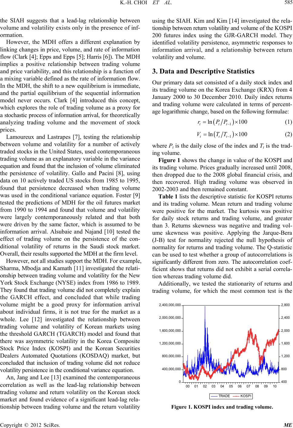
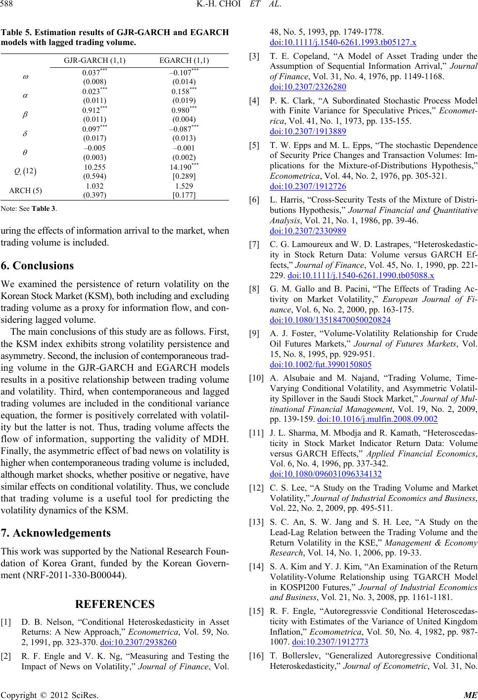
Table 5. Estimation results of GJR-GARCH and EGARCH
models with lagged trading volume.
GJR-GARCH (1,1) EGARCH (1,1)

0.037***
(0.008)
–0.107***
(0.014)

0.023***
(0.011)
0.158***
(0.019)

0.912***
(0.011)
0.980***
(0.004)

0.097***
(0.017)
–0.087***
(0.013)

–0.005
(0.003)
–0.001
(0.002)

12
s
Q 10.255
(0.594)
14.190***
[0.289]
ARCH (5) 1.032
(0.397)
1.529
[0.177]
Note: See Table 3.
uring the effects of information arrival to the market, when
trading volume is included.
6. Conclusions
We examined the persistence of return volatility on the
Korean Stock Market (KSM), both including and excluding
trading volume as a proxy for information flow, and con-
sidering lagged volume.
The main conclusions of this study are as follows. First,
the KSM index exhibits strong volatility persistence and
asymmetry. Second, the inclusion of contemporaneous trad-
ing volume in the GJR-GARCH and EGARCH models
results in a positive relationship between trading volume
and volatility. Third, when contemporaneous and lagged
trading volumes are included in the conditional variance
equation, the former is positively correlated with volatil-
ity but the latter is not. Thus, trading volume affects the
flow of information, supporting the validity of MDH.
Finally, the asymmetric effect of bad news on volatility is
higher when contemporaneous trading volume is included,
although market shocks, whether positive or negative, have
similar effects on conditional volatility. Thus, we conclude
that trading volume is a useful tool for predicting the
volatility dynamics of the KSM.
7. Acknowledgements
This work was supported by the National Research Foun-
dation of Korea Grant, funded by the Korean Govern-
ment (NRF-2011-330-B00044).
REFERENCES
[1] D. B. Nelson, “Conditional Heteroskedasticity in Asset
Returns: A New Approach,” Econometrica, Vol. 59, No.
2, 1991, pp. 323-370. doi:10.2307/2938260
[2] R. F. Engle and V. K. Ng, “Measuring and Testing the
Impact of News on Volatility,” Journal of Finance, Vol.
48, No. 5, 1993, pp. 1749-1778.
doi:10.1111/j.1540-6261.1993.tb05127.x
[3] T. E. Copeland, “A Model of Asset Trading under the
Assumption of Sequential Information Arrival,” Journal
of Finance, Vol. 31, No. 4, 1976, pp. 1149-1168.
doi:10.2307/2326280
[4] P. K. Clark, “A Subordinated Stochastic Process Model
with Finite Variance for Speculative Prices,” Economet-
rica, Vol. 41, No. 1, 1973, pp. 135-155.
doi:10.2307/1913889
[5] T. W. Epps and M. L. Epps, “The stochastic Dependence
of Security Price Changes and Transaction Volumes: Im-
plications for the Mixture-of-Distributions Hypothesis,”
Econometrica, Vol. 44, No. 2, 1976, pp. 305-321.
doi:10.2307/1912726
[6] L. Harris, “Cross-Security Tests of the Mixture of Distri-
butions Hypothesis,” Journal Financial and Quantitative
Analysis, Vol. 21, No. 1, 1986, pp. 39-46.
doi:10.2307/2330989
[7] C. G. Lamoureux and W. D. Lastrapes, “Heteroskedastic-
ity in Stock Return Data: Volume versus GARCH Ef-
fects,” Journal of Finance, Vol. 45, No. 1, 1990, pp. 221-
229. doi:10.1111/j.1540-6261.1990.tb05088.x
[8] G. M. Gallo and B. Pacini, “The Effects of Trading Ac-
tivity on Market Volatility,” European Journal of Fi-
nance, Vol. 6, No. 2, 2000, pp. 163-175.
doi:10.1080/13518470050020824
[9] A. J. Foster, “Volume-Volatility Relationship for Crude
Oil Futures Markets,” Journal of Futures Markets, Vol.
15, No. 8, 1995, pp. 929-951.
doi:10.1002/fut.3990150805
[10] A. Alsubaie and M. Najand, “Trading Volume, Time-
Varying Conditional Volatility, and Asymmetric Volatil-
ity Spillover in the Saudi Stock Market,” Journal of Mul-
tinational Financial Management, Vol. 19, No. 2, 2009,
pp. 139-159. doi:10.1016/j.mulfin.2008.09.002
[11] J. L. Sharma, M. Mbodja and R. Kamath, “Heteroscedas-
ticity in Stock Market Indicator Return Data: Volume
versus GARCH Effects,” Applied Financial Economics,
Vol. 6, No. 4, 1996, pp. 337-342.
doi:10.1080/096031096334132
[12] C. S. Lee, “A Study on the Trading Volume and Market
Volatility,” Journal of Industrial Economics and Business,
Vol. 22, No. 2, 2009, pp. 495-511.
[13] S. C. An, S. W. Jang and S. H. Lee, “A Study on the
Lead-Lag Relation between the Trading Volume and the
Return Volatility in the KSE,” Management & Economy
Research, Vol. 14, No. 1, 2006, pp. 19-33.
[14] S. A. Kim and Y. J. Kim, “An Examination of the Return
Volatility-Volume Relationship using TGARCH Model
in KOSPI200 Futures,” Journal of Industrial Economics
and Business, Vol. 21, No. 3, 2008, pp. 1161-1181.
[15] R. F. Engle, “Autoregressvie Conditional Heteroscedas-
ticity with Estimates of the Variance of United Kingdom
Inflation,” Ecomometrica, Vol. 50, No. 4, 1982, pp. 987-
1007. doi:10.2307/1912773
[16] T. Bollerslev, “Generalized Autoregressive Conditional
Heteroskedasticity,” Journal of Econometric, Vol. 31, No.

K.-H. CHOI ET AL.
589
3, 1986, pp. 307-327. doi:10.1016/0304-4076(86)90063-1
[17] L. R. Glosten, R. Jagannathan and D. E. Runkle, “On the
Relation between the Expected Value and the Volatility
of the Nominal Excess Return on Stocks,” Journal of Fi-
nance, Vol. 48, No. 5, 1993, pp. 1779-1801.
doi:10.1111/j.1540-6261.1993.tb05128.x