Modern Economy, 2012, 3, 526-533
http://dx.doi.org/10.4236/me.2012.35069 Published Online September 2012 (http://www.SciRP.org/journal/me)
A Simple Trade Model with an Optimal Exchange Rate
Motivated by Discussion of a Renminbi Float*
Hui Huang1, Yiming Wang2, Joh n Whalley3, Shunming Zhang4
1Faculty of Business Administration, The University of Regina, Regina, Canada
2Department of Finance, School of Economics, Peking University, Beijing, China
3Department of Economics, Social Science Centre, The University of Western Ontario, London, Canada
4China Financial Policy Research Center, School of Finance, Renmin University of China, Beijing, China
Received March 22, 2012; revised April 25, 2012; accepted May 8, 2012
ABSTRACT
We present a model of combined inter-sp atial and inter-temporal trade between countries in which there is a fixed ex-
change rate with a surrender requirement for foreign exchange generated by exports. The model incorporates inter-
temporal intermediation services, which may or may not be liberlized across countries. We use numerical simulation
methods to explore the properties of the model, since it has no closed form solution. In this model, when services re-
main unliberalized there is an optimal trade intervention, even in the small open price taking economy case. Given
monetary policy and an endogenously determined premium value on foreign exchange, an optimal setting of the ex-
change rate can provide the opti mal trade intervention. We suggest th is model may have loose relevance for the current
situation in China where services remain unliberalized and tar iff rates are bound in the WTO and a free Renminbi float
is under discussion.
Keywords: Fixed Exchange Rate; Foreign Exchange Premium; Services; JEL Classification: F00; F02; F31; F32
1. Introduction
This paper takes as its point of departure macro literature
on the choice of exchange rate regime. While the choice
between a fixed and flexible exchange rate regime has
long been argued and debated in classical monetarist t erms
(that a fixed exchange rate implies accommodating mone-
tary policy, and monetary policy determines the floating
rate) as in Friedman’s [1] discussion, there is little litera-
ture that suggests t hat there may exi st an opt imal exchange
rate which dominates a free float1.
We use a model of combined inter-spatial and inter-
temporal trade between countries in which there is a fix ed
exchange rate accompanied by a surrender requirement
for foreign ex change g enerated by expor ters. Huang, Whal-
ley and Zhang [4] earlier analyzed the merits of trade
liberalizatio n i n finan cial services using a related appr oach
both with no treatment of the exchange rate require. In
their model, in the presen ce of tariffs o n inter-spati al t ra de
free trade in services, even for a small open price taking
economy, may not be welfare improving, and free trade
in goods may not be Pareto optimal if services trade re-
mains unliberalized.
In the model presented here, under either auctioning of
foreign exchange received by the central bank among im-
porters, or some non auctioned foreign exchange alloca-
tion mechanism with domestic trading in foreign exchange,
there will be a premium value on foreign exchange which
is endogenously determined and operates akin to a tariff
on imports. In simple models where income effects among
consumers are assumed away, domestic monetary policy
in such a model is non neutral, while trade liberalization
(a tariff reduction) merely changes the premium value on
foreign exchange, leaving trade unchanged. Since mone-
tary policy is n on-neu tral, when services re main unlibe ra l-
ized there is an optimal trade intervention, even in the
small economy case. This occurs because given monetary
1Such a contention is relevant to current policy debate in China, since
with an optimal exchange rate a freely floating rate may be welfare
worsening. China has long maintained a fixed exchange rate with tight
regulation of domestic banks, and strict limits on entry to the Chinese
market for foreign financial institutions. In past, this has reflected a
desire for macro stability, but the Chinese banking system also differs
sharply from those in OECD countries with small but growing personal
banking, and state owned banks acting in part as mechanisms for recapit-
alizing loss making state owned enterprises. Thus, much of what is at
state in the debate on financial liberalization in China and the choice o
f
exchange rate regime is the form and operation of the Chinese banking
system and how this would change with a freely floating fully conve-
rt ib le Ren minbi and this goes well beyond the discus sion here (se e Z ha ng
and Pan [2] and Chang and S h ao [3]).
*This work is supported form National Natural Science Foundation o
f
China (NSFC Grant: 70825003) and National Social Science Found-
ation of China (SSFC Grant: 07AJL002).
C
opyright © 2012 SciRes. ME

H. HUANG ET AL. 527
policy and an endogenously determined premium value
on foreign exchange, an optimal setting of the exchange
rate can provide the optimal trade intervention. Under a
freely floating exchange rate any departure from this
optimal rate will typically inflict welfare losses. In a two
country model, a retaliatory exchange rate game, related
to well known tariff games can be constructed, fo r which
a Nash equilibrium in exchange rates can be computed.
We present the model, and illustrate possib le outcomes
using numerical simulation, and discuss its relevance to
the contempor ar y Ch ines e s itua tion wher e serv ice s ar e unl i-
beralized and tariffs are bound in the WTO. We would
not pretend that th is model realistical ly cap tu res all of th e
relevant features of the financial and real sides of the Ch i-
nese economy, and hence may only be suggestive in its
implications for current policy. Importantly, there is no
foreign exchange premium in China since China is cur-
rentl y runn ing a trad e surp lus ra ther th an th e balan ced trade
our model specifies, and concerns over potential capital
flight under a free float are the most important factor in
current debates and they are not captured here. But the
implication that if services remain largely unliberalized
(as in China today) and tariff rates are bound in the WTO
a move to a free float may be welfare worsening in our
analysis seems both clear and relevant, and should be kep t
in mind by those currently advocating a free Renminbi
float.
2. A Model of Spatial and Inter-Temporal
Trade with a Fixed Exchange Rate and
Non-Neutral Monetary Policy
We consider a world in which two types of trade are pos-
sible. One is inter-spatial trade between countries in com-
modities, and the other inter-tempor al trade facilitated by
providers of intermediation services. To simplify things,
we further assume tha t intermediation serv ices, when t hey
are provided, are supplied at zero cost to users of services,
and also that such services can only be provided by for-
eign service providers. This gross simplification implies
that all intertemporal trade implies international trade in
intermediation services, but adopting it means that we can
consider autarky in services to be a case where no inter-
temporal intermediatio n occu rs, and free trade in services
to be the case where full inter-temporal intermediation
occurs. If services remain unliberalized budget constraints
within each period hold when we consider changes in
exogenous variable (such as fixed exchange rates) in the
model. We do not claim that this is a realistic representa-
tion of how service sectors operate in actual economies,
but it is a useful analytical si mplification.
We assume a fixed exchange rate regime with result-
ing monetary non-neutralities. We assume domestic cur-
rency is needed to execute domestic transactions while
foreign currency is both needed for purchases of imports
and yielded by the sale of exports. We only consider the
transaction demand for money and in our formulation all
foreign exchang e earni ngs of expor ter s are su rrend ere d to
the central bank at the fixed exchange rate, while foreign
exchange received by the bank is auctioned among im-
porters at a premium to the official exchange rate. This
premium value is endogenously determined given mone-
tary policy, and operates akin to a tariff. (Also see Clarete
and Whalley [5]).
For simplicity, we consider the 2 period (t = 0, 1), 1
country, 2 good (l = 1, 2) pure exchange international
trade case of a small open price taking economy. Adding
additional features such as produc tion, or more periods or
goods, merely complicates the analysis while the themes
remain the same.
The model can be presented as follows. The country
has a single representative consumer, with endowments
of the two goods in each period (l; t = 0, 1, l = 1, 2),
and inter-temporal preferences written as
t
E


 
1
12
=0
000 111
12 12
1
=,
1
1
=, ,
1
ttt
t
t
UuXX
uXX uXX





t
l
(1)
where ρ is inter-temporal discount factor and
X
de-
notes consumption of good l at date t.
If a time-additive Cobb-Douglas utility fu nction of the
form

12
12 12
,= tt
tttt t
uXXX X



 
  for t = 0, 1 is

used, (1) can be represented more explicitly as
00 11
12 12 00 11
12 12
1
=1 UXXX X




 


 

t
l
(2)

is the share parameter for good l at date t where


2=1
t


t
=1 l l
For good l in each period t, the exogenous world price
is l
. We can also consider CES preferences.

. We allow the country to impose tariffs at rate l
on each imported good l (i.e. if ll
t
T
tt
X
E0T
tt
, then t
l).
Tariffs are set to equal zero if good l is exported (i.e. if
ll
X
E

, then l0
t
T

). Internal (gross of tariff) prices
for good l at date t are thus


=1 ,=0,1,=1,2
tt t
lll
PTtl

2
=1
=,=0,1
ttttt
ll ll
l
RTXEt



t
E
2
=1
=,=0,1
tttt
ll
l
IPERt

. (3)
These are also sellers prices of good l.
Tariff revenues collected in period t are
(4)
where l denotes the initial endowment of good l. In-
come in period t is given by
. (5)

H. HUANG ET AL.
528
We consider the case in which both goods are traded,
and there is both a fixed exchange rate and rationed for-
eign exchange. We assume that the government fixes the
exchange rate at et, and requires all foreign exchange
earned by exporters to be surrendered to the Central Ba nk
at the rate et. It then allocates rights to purchase available
foreign exchange to importers at the same rate et. We will
assume that exporters comply with this policy and fully
meet the surrender requirement, even though there are ob-
vious incentives for exporters to conceal foreign exchan ge
and attempt to sell it on parallel (black) markets rather
than surrender it at the lower fixed rate. The allocation
process of foreign exchange among importers assumes
that the government auctions (or sells) foreign exchange.
In practice, allocation schemes actually followed are mor e
complex than this involving priority allocation of various
forms, but we abstract from these. But under such a sim-
ple auctioning scheme, if desired imports require more
foreign exchange than the government offers for sale, th e
price of foreign exchange paid by importers will be bid
up. This price will thus include a foreign exchange pre-
mium above the fixed rate et, which we designate as λt.
This premium acts as a surcharge on foreign exchange
bought by importers, and adjusts so as to clear the for-
eign exchange market.
In this formulation the net effect of foreign exchange
rationing is similar to a tariff on all imports, since the ex-
change rate received by exporters differs from the gross
of premium value exchange rate paid by importers. The
difference from a tariff is that the premium rate (or tariff
equivalent rate) is endogenously determined. Also, under
an auctioning scheme, the foreign exchange premium ac-
crues to the government, but if rights to purchase foreign
exchange at the rate et were instead allocated by the gov-
ernment without charge, the premium would instead go
directly to importers.
The world prices for the 2 goods are given as l
t

for
t = 0, 1 and l = 1, 2. Domestic prices (gross of tariff and
gross of the foreign exchange premium for imports) for
the 2 goods are again denoted as for t = 0, 1 and l =
1, 2, and are defi ned belo w b y (7).
t
l
P
Assuming unitary velocity of circulation and that the
only demand for money is for transaction purposes, the
demand for domestic currency t
D
M
at date t is given by
the value of domestic demands in domestic currency, i.e.
2
=1
tt
Dl
l
MP

=,=0,1
t
l
Xt
t
(6)
Implicitly, we assume that imports are bought by mid-
dle men (imports) using foreign currency, who then im-
port costlessly and sell imports at domestic prices. The s up -
ply of domestic currency at date t is assumed to be set by
the domestic monetary authorities and is given by S
M
.
Because of the foreign exchange premium, relative do-
mestic prices of the 2 traded goods will now differ from
world prices both due to the premium on foreign exchange
and the tariff, depending upon whether the good is im-
ported or exported. Domestic prices l gross of the for-
eign exchange premium are thus now given by
t
P

,0
=1, >0
ttt t
lll
t
ltttt t
lll
eifXW
PeifXW



 


tt
(7)
where ll
X
W
t
denotes the net import of goods l, and λt
is the premiu m value over the officia l exchang e rate paid
by purchasers of imports.
The demand for foreign currency
D
N
2
=1
=,=0,1.
tttt
Dlll
l
NXWt





t
N
2
=1
=,=0,1.
tttt
Slll
l
NXWt





=
tt
at date t is given
by the value of imports at world prices
(8)
The supply of foreign currency S at date t is given
by the value of exports at world prices
(9)
We consider two types of equilibrium. One of these is
characterized by no provision of intermediation services
by foreign services providers, and since we assume them
to be the on ly po tent ial se rvic e provid ers, no inte r-te m pora l
intermediation. In this equilibrium, period by period b u d g et
constraints apply for the economy, and we associate such
an equilibrium with autarky in services trade. The other
type of equilibrium is characterized by costless interna-
tional flows of intermediation services (or free trade in s er -
vices), and in this case combined period by period budget
constraints hold. The only role for foreign services pro-
viders in the model is to costlessly facilitate intermedia-
tion within the price taking economy.
If there is no trade in intermediation services trade bal-
ance holds in each period, which implies that the value of
imports goods is equal to the value of export and hence
D
S
NN
2
=1 =0.
tt t
ll l
l
XW




2
=1
=,=0,1
ttt tt t
ll l
l
ReXW t 





for t = 0, 1. Trade balance implies that
(10)
which also implies that total revenues accruing to sellers
of rights to purchase foreign exchange at the rate et are
(11)
These revenues accrue either directly to the household
sector as additional income of importers who are given
allocations of foreign exchange by the government which
they resell on premium markets, or indirectly as recycled
government reve nu e s . Be cause anti cipated revenues Lt from
rights of access to foreign exchange affect commodity de-
mands and are a component of income for at least one of

H. HUANG ET AL. 529
the agents in the model, market demand functions have to
be rewrit ten to reflect this. Bo th Lt and Rt are each e nd og e-
nously determined , a nd Lt = Rt only in equilibrium.
The budget constraint for the household sector in this
case includes initial holdings of money balances, and is
given by
2
=1
=
ttt
llS
l
IPWM
,=0,1
tt
Lt
=, =0,1
t
I t
=,=0,1
t
L t

=0,
tt
RL

,
tt
L 

0,1;=1,2l
22
..=, =0,1
ttttttt
st P XMPWMLt

2
=1 =0
=0 =0
tttt
ll l
l
ttt t
DS
eXWand
RLandM M





=
tt
(12)
2.1. General Equilibrium with Service Trade
Autarky (Period by Period Budget
Constraints)
When there is service trade autarky no intermed iation ser-
vices are provided since by assumption there are no do-
mestic service providers2. This means that there is incom-
pleteness in the coverage of markets in the sense that in
service trade autarky intertemporal markets are missing.
This enables us to appeal directly to literature on multi-
commodity inter-temporal models of incomplete markets
due to Radner [10], Hart [11], Duffie and Shafer [12],
Werner [13], Duffie [14], Geanakopolos [15], Magill and
Shafer [16], and Magill and Quinzii [17] in analyzing the
effects of service liberalization in this model. In services
trade autarky there is no inter-temporal trade, while with
costless inter-temporal trade in services inter-temporal
markets are complete. We use incomplete markets litera-
ture without the added complication of uncertainty; most
of this literature is concerned with existence issues; our
focus here is comparative statics.
In the absence of trade in financial intermediation ser-
vices the total value of expenditures must satisfy the
household budget constraint in each period, i.e.,
2
=1
tt t
llD
l
PX M
 (13)
that is,
22
=1 =1
tt ttt t
ll DllS
ll
PX MPWM
 (14)
or

2
=1
=0 ,1
ttttt t
ll lDS
l
eXWMM
t



(15)
A single country equilibrium in this case is given by
values of which satisfy the conditions:
1) solves :=
t
l
Xt
maxU
=1 =1
ll Dll S
ll
(16)
2) For t = 0, 1, trade balance, premium revenue bal-
ance, and money demand and supply equalities hold in each
period.
(17)
2) Implies that
D
S
NN

for t = 0, 1.
2.2. General Equilibrium with Free Trade in
Services (Across Period Budget Constraints)
If costlessly provided foreign supplied intermediation ser-
vices are allowed in the model, then we can characterize
a free trade in services equilibrium as a case where ac ros s
period budget constraints hold rather than period by pe-
riod budget constraints. In this model form, we assume
the interest rate r is endogenously determined on the
country capital market to clear demand for and supply of
loans. The economy is then only a price taker in goods
markets, and foreign financial intermediaries only prov ide
their services to the single country.
In this case, the demand for foreign currency is
1
=0
=1
t
D
Dt
t
N
N
r


. The supply of for eign currency is
1
=0
=1
t
S
St
t
N
N
r

=
. Trade balance now implies that the
value of imports equals the value of exports and
D
S
NN

,
i.e.
12
=0 =1
22
00011 1
=1 =1
1
1
1
==0.
1
tt t
ll l
t
tl
lllll l
ll
XW
r
XW XW
r




 
 
 




20000
=1
2111 1
=1
=
=1
ll D
l
ll D
l
PXMFI
PXMIr F










22
00 000 00
=1 =1
22
11 111 11
=1 =1
=
=1
ll DllS
ll
ll DllS
ll
PX MFPW M L
PXMPWMLr F
 








(18)
With trading now allowed across the 2 periods under
liberalized trade in financial intermediation services, the
total value of expenditures satisfy the household budget
constraint in each period, including borrowing and lend-
ing across periods, i.e.,
(19)
where following the literature on incomplete markets F is
the amount of credit extended across periods by foreign
finance service providers. (19) can be rewritten as
(20)
2See the discussion of barriers to trade in intermediation services in
p
ractice in Chen and Schembri [6], Francois and Schuknecht [7], Ka-
lirajan, McHuire, Nguyen and Schuele [8], and Mattoo [9].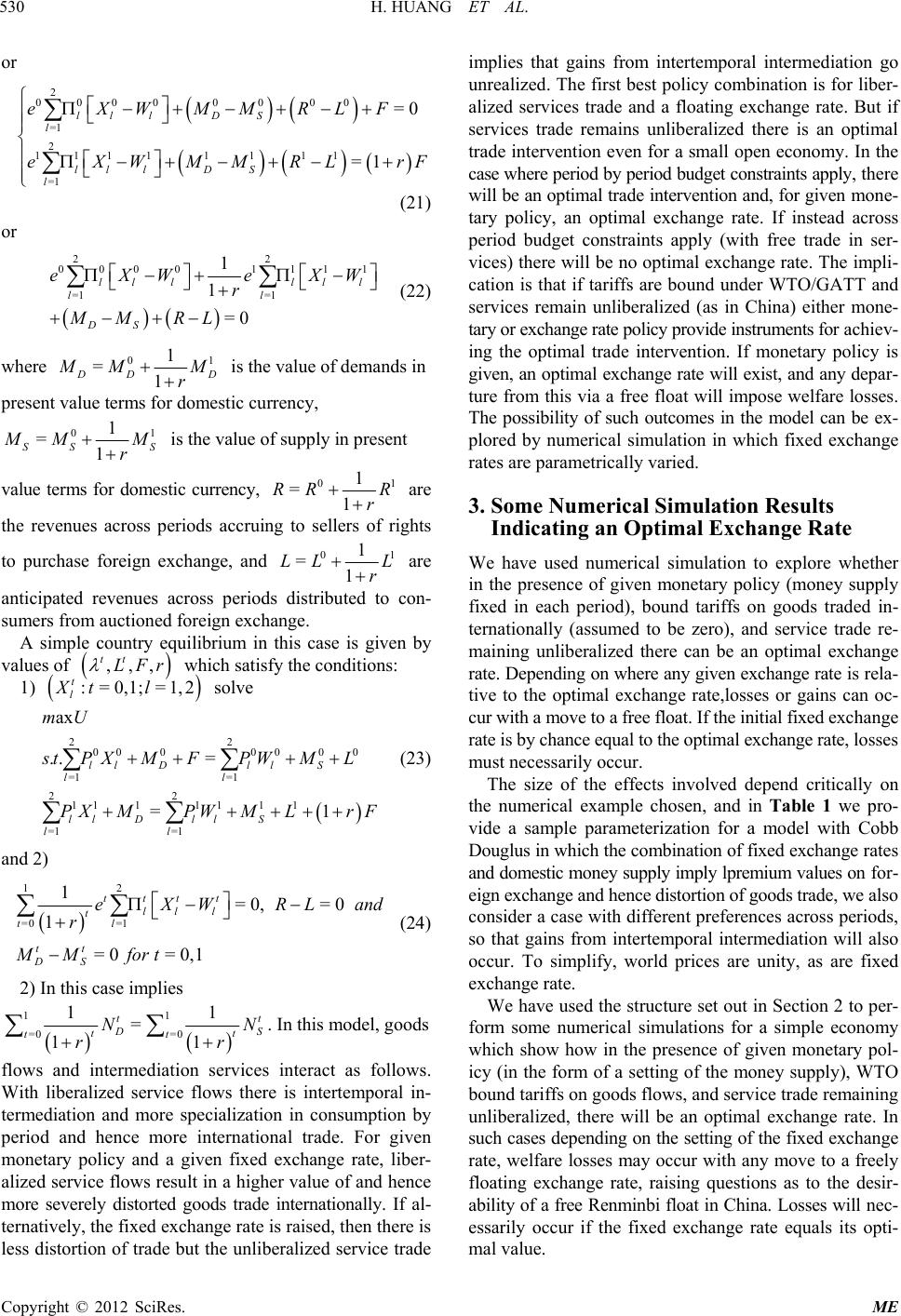

H. HUANG ET AL.
530
or


2
00000 00
=1
2
11111 11
=1
ll lDS
l
ll lD S
l
eXWMM
eXWMMR















0
1
=0
=1
RLF
L rF

 
(21)
or
 
22
0000 1
=1 =1
1
1
=0
lll
ll
DS
eXW e
r
MM RL






111
ll l
XW



(22)
where 01
1
1
=
D
DD
M
MM
r
 is the value of demands in
present value terms for domestic currency,
01
1
1
SS S
=
M
MM
r
 is the value of supply in present
value terms for domestic currency, 01
1
1
RR R
r
 = are
the revenues across periods accruing to sellers of rights
to purchase foreign exchange, and 01
1
=1 LL L
r
 are

anticipated revenues across periods distributed to con-
sumers from auctioned foreign exchange.
A simple country equilibrium in this case is given by
values of which satisfy the conditions:

,,,
tt
LFr 

0,1;=1,2l

000
11
l S
M L
LrF


1) solve :=Xt
axmU
t
l
22
00 00
=1 =1
22
11 111 1
=1 =1
.. =
=
ll Dl
ll
ll DllS
ll
st PXMFP W
PX MPW M




(23)
and 2)

12
=0 =1
1=0,
1
=0 =0,1
tttt
ll l
t
tl
tt
DS
eX WR
r
MM fort





 =0L and
(24)
2) In this case implies
 
1
=0
1
=1
=0
1
11
tt
D
S
t t
NN
rr

t t
. In this model, goods
flows and intermediation services interact as follows.
With liberalized service flows there is intertemporal in-
termediation and more specialization in consumption by
period and hence more international trade. For given
monetary policy and a given fixed exchange rate, liber-
alized service flows result in a higher value of and hence
more severely distorted goods trade internationally. If al-
ternatively, the fixed exchange r ate is r a ised, then there is
less distortion of trade but the unliberalized service trade
implies that gains from intertemporal intermediation go
unrealized. The first best policy combination is for liber-
alized services trade and a floating exchange rate. But if
services trade remains unliberalized there is an optimal
trade intervention even for a small open economy. In the
case where per iod by period budget con straints apply, t h er e
will be an optimal trade intervention and, for given mone -
tary policy, an optimal exchange rate. If instead across
period budget constraints apply (with free trade in ser-
vices) there will be no optimal exchange rate. The impli-
cation is that if tariffs are bound under WTO/GATT and
services remain unliberalized (as in China) either mone-
tary or exchange rate policy provide instruments for achiev-
ing the optimal trade intervention. If monetary policy is
given, an optimal exchange rate will exist, and any dep ar-
ture from this via a free float will impose welfare losses.
The possibility of such outcomes in the model can be ex-
plored by numerical simulation in which fixed exchange
rates are parametrically varied.
3. Some Numerical Simulation Results
Indicating an Optimal Exchange Rate
We have used numerical simulation to explore whether
in the presence of given monetary policy (money supply
fixed in each period), bound tariffs on goods traded in-
ternationally (assumed to be zero), and service trade re-
maining unliberalized there can be an optimal exchange
rate. Depending on where any given exchange rate is r el a-
tive to the optimal exchange rate,losses or gains can oc-
cur with a move to a free float. If the initial fixed exchange
rate is by chance equal to the optimal exchange rate, losses
must necessarily occur.
The size of the effects involved depend critically on
the numerical example chosen, and in Table 1 we pro-
vide a sample parameterization for a model with Cobb
Douglus in which the combination of fixed exchange r at e s
and domestic money supply imply lpremium values on f o r -
eign exchange and hence distortion of goods trade, we also
consider a case with different preferences across periods,
so that gains from intertemporal intermediation will also
occur. To simplify, world prices are unity, as are fixed
exchange rate.
We have used the structure set out in Section 2 to per-
form some numerical simulations for a simple economy
which show how in the presence of given monetary pol-
icy (in the form of a setting of the money supply), WTO
bound tariffs on goods flows, and service trade remaining
unliberalized, there will be an optimal exchange rate. In
such cases depending on the setting of the fixed exchan ge
rate, welfare losses may occur with any move to a freely
floating exchange rate, raising questions as to the desir-
ability of a free Ren minbi float in China. Losses will n ec-
essarily occur if the fixed exchange rate equals its opti-
mal value.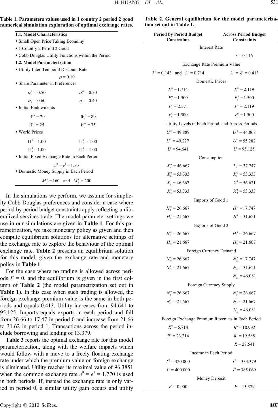

H. HUANG ET AL. 531
Table 1. Parameters values used in 1 country 2 period 2 good
numerical simulation exploration of optimal exchange rates.
1.1. Model Characteristics
 Small Open Price Taking Economy
 1 Country 2 Per iod 2 Go o d
 Cobb Douglas Utility Functions within the Period
1.2. Model Parameterization
 Utility Inter-Temporal Discount Rate
=0.10

 Share Parameter in Preferences
0
1=0.5

0
2=0.50

1
1=0.6

1
2=0.40

0
1=20W0 2=80W
1
1=25W1 2=75W
0
1=1.00 2=1.00
1=1.01=1.00
01
= =1.50ee
1=200
S
M
0
0
 Initial Endowments
 World Prices
0
1 2
 Initial Fixed Exchange Rate in Each Period
0
 Domestic Money Supply in Each Period
0=160
S
M and
In the simulations we perform, we assume for simplic-
ity Cobb-Douglas preferences and consider a case where
period by period budget constraints apply reflecting u nl ib-
eralized services trade. The model parameter settings we
use in our simulations are given in Table 1. For this pa-
rametrization, we take monetary policy as given and then
compute equilibrium solutions for alternative settings of
the exchange rate to explore the behaviour of the optimal
exchange rate. Table 2 presents an equilibrium solution
for this model, given the exchange rate and monetary
policy in Table 1.
For the case where no trading is allowed across peri-
ods F = 0, and the equilibrium is given in the first col-
umn of Table 2 (the model parametrization set out in
Table 1). In this case when such trading is allowed, the
foreign exchange premium value is the same in both pe-
riods and equals 0.413. Utility increases from 94.641 to
95.125. Imports equals exports in each period and fall
from 26.66 to 17.47 in period 0 and increase from 21.66
to 31.62 in period 1. Transactions across the period in-
clude borrowing and lending of 13.379.
Table 3 reports the optimal exchange rate for this mo d el
parameterization, along with the welfare impacts which
would follow with a move to a freely floating exchange
rate under which the premium value on foreign exchange
is eliminated. Utility reaches its maximal value of 96.38 51
when the common exchange rate e0 = e1 = 1.770 is used
in both periods. If, instead the exchange rate is only var-
ied in period 0, a similar utility gain occurs and utility
Table 2. General equilibrium for the model parameteriza-
tion set out in Table 1.
Period by Period Budget
Constraints Across Period Budget Constraints
Interest Rate
= 0.116r
0=0.143

1=0.714

01
==0.413 
0
1=1.714P0 1= 2.119P
0
2=1.500P0 2=1.500P
1
1=2.571P1 1=2.119P
1
2=1.500P1 2=1.500P
0= 49.889U0= 44.868U
1= 49.227U1= 55.282U
= 94.641U= 95.125U
0
1= 46.667X0 1= 37.747X
0
2= 53.333X0 2= 53.333X
1
1=46.667X1 1=56.621X
1
2= 53.333X1 2= 53.333X
0
1= 26.667H0 1=17.747H
1
1=21.667H1 1= 31.621H
0
2= 26.667H0 2= 26.667H
1
2=21.667H1 2=21.667H
0=26.667
D
N0=17.747
D
N
1= 21.667
D
N1= 31.621
D
N
=46.081
D
N
0= 26.667
S
N0=26.667
S
N
1=21.667
S
N1=21.667
S
N
= 46.081
S
N
0=5.714R0=10. 992R
1= 23.214R1=19.585R
= 28.541R
0= 320.000I0= 333.379I
1= 400.000I1=385.069I
=0.000F=13.379F
Exchange Rate Premium Value
and
Domestic Prices
Utility Levels in Each Period, and Across Periods
Consumption
Imports of Good 1
Exports of Good 2
Foreign Currency Demand
Foreign Currency Supply
Foreign Exchange Premium Revenues in Each Period
Income in Each Period
Money Deposit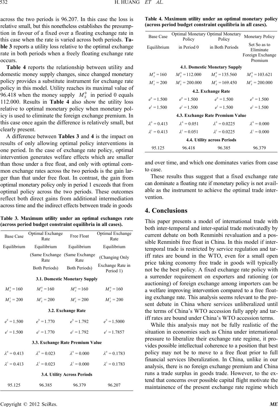

H. HUANG ET AL.
532
across the two periods is 96.207. In this case the loss is
relative small, but this nonetheless establishes the pres u m p-
tion in favour of a fixed over a floating exchange rate in
this case when the rate is varied across both periods. Ta-
ble 3 reports a utility loss relative to the optimal excha ng e
rate in both periods when a freely floating exchange rate
occurs.
Table 4 reports the relationship between utility and
domestic money supply changes, since changed monetary
policy provides a substitute instrument for exchange rate
policy in this model. Utility reaches its maximal value of
96.418 when the money supply S
0
M
in period 0 equals
112.000. Results in Table 4 also show the utility loss
relative to optimal monetary policy when monetary pol-
icy is used to eliminate the foreign exchange premium. In
this case once again the difference is relatively small, but
clearly present.
A difference between Tables 3 and 4 is the impact on
results of only allowing optimal policy interventions in
one period. In the case of exchange rate policy, optimal
intervention generates welfare effects which are smaller
than those under a free float, and only with optimal com-
mon exchange rates across the two periods is the gain lar -
ger than that under free float. In contrast, the gain from
optimal monetary policy only in period 1 ex ceeds that f r om
optimal policy across the two periods. These outcomes
reflect both direct gains from additional intermediation
across time and the indirect effects between trade in goods
Table 3. Maximum utility under an optimal exchanges rate
(across period budget constraint equilibria in all cases).
Base Case Optimal Exchange
Rate Free Float Optimal Exchange
Rate
Equilibrium Equilibrium Equilibrium Equilibrium
(Same Exchange
Rate (S ame Excha nge Rate (Changing On ly
Both Periods) Both Periods) Exchange Rate in
Period 1)
3.1. Domestic Monetary Supply
0=160
S
M 0=160
S
M 0=160
S
M
Table 4. Maximum utility under an optimal monetary policy
(across period budget constraint equilibria in all cases).
Base CaseOpti mal Monetary
Policy Optimal Monetary Policy Monetary Policy
Equilibriumin Period 0 in Both Periods Set So as to
Eliminate
Foreign Exchange
Premium
4.1. Domestic Monetary Supply
0=160
S
M0=112.000
S
M0=135.560
S
M0=103.621
S
M
1=200
S
M1= 200.000
S
M1=169.450
S
M1= 200.000
S
M
0=1.500e0=1.500e0=1.500e0=1.500e
1=1.500e1=1.500e1=1.500e1=1.500e
0=0.413

0= 0.051

0=0.0225

0=0.000

1=0.413

1=0.051

1=0.0225

1=0.000

4.2. Exchange Ra te
4.3. Exchange Rate P r emium Value
4.4. Utility across Periods
95.125 96.418 96.385 96.379
and over time, and which one dominates varies from case
to case.
These results thus suggest that a fixed exchange rate
can dominate a f loating r ate if mo netar y policy is not a v ai l -
able as the instrument to achieve the optimal trade inter-
vention.
4. Conclusions
This paper presents a model of international trade with
both inter-temporal and inter-spatial trade motivatedly by
current debate on both Renminbi revaluation and a pos-
sible Renminbi free float in China. In this model if inter-
temporal trade is restricted by service regulation and tar-
iff rates are bound in the WTO, even for a small open
price taking economy free trade in goods will typically
not be the best policy. A fixed exchange rate policy with
a surrender requirement on exporters and rationing (or
auctioning) of foreign exchange among importers can be
a welfare improving intervention compared to a free float-
ing exchange rate. This analysis seems relevant to the p re -
sent debate in China where services unliberalized until
the terms of China’s WTO accession fully apply and tar-
iff rates are bound under China’s WTO accession terms.
0=160
S
M
1=200
S
M
0=1.5000e
1=1.7857e
0=0.1783

1=0.1783

1=200
S
M 1=200
S
M 1=200
S
M
3.2. Exchange Ra te
0=1.500e 0=1.770e 0=1.792e
1=1.500e 1=1.770e 1=1.792e
3.3. Exchange Rate P r emium Value
0=0.413
 0=0.023  0=0.000 
1=0.413
 1=0.023  1=0.000 
3.4. Utility Across Periods
95.125 96.385 96.379 96.207
While this analysis may not be fully realistic of the
situation in economies such as China under international
pressure to liberalize their exchange rate regime, it pro-
vides possible intellectual coherence to a position that be st
policy may not be to move to a free float prior to full
financial services liberalization. In China, unlike in our
analysis, there is no foreign exchange premium and Chin a
runs a trade surplus in goods trade. However, to the ex-
tend that concerns over possible capital flight motivate t he
maintainence of the present exchange rate regime which

H. HUANG ET AL.
533
limits convertability, the broad themes of the analysis sti ll
seem relevant. The policy implications thus run counter
to accepted international conventional wisdom and point
to possible advantag es of not freely floating.
REFERENCES
[1] M. Friedman, “Essays in Positive Economics,” Chapter
on the Case for Flex Exchange Rate, 1956.
[2] Z. Pan and F. Zhang, “Determination of China’s Long-
Run Nominal Exchange Rate and Official Intervention,”
China Economic Review, Vol. 15, No. 3, 2004, pp. 360-
365. doi:10.1016/j.chieco.2004.04.002
[3] G. Chang and Q. Shao, “How Much Is the Chinese Cur-
rency Undervalued? A Quantitative Estimation,” China
Economic Review, Vol. 15, No. 3, 2004, pp. 366-371.
[4] H. Huang, J. Whalley and S. Zhang, “Trade Liberaliza-
tion in a Joint Spatial Inter-Temporal Trade Model,” Re-
search Paper, The University of Western Ontario, 2004.
[5] R. Clarete and J. Whalley, “Foreign Exchange Premia and
Non-Neutrality of Monetary Policy in General Equilib-
rium Models,” Journal of International Economics, Vol.
30, No. 1-2, 1991, pp. 153-166.
[6] Z. Chen and L. Schembri, “Measuring the Barriers to
Trade in Services: Literature and Methodologies,” In: J.
M. Curtis and D. C. Ciuriak, Eds., Trade Policy Research,
Development of Foreign Affairs and International Trade,
2002.
[7] J. Francois and L. Schuknecht, “International Trade in
Financial Services, Competition and Growth Perform-
ance,” Centre for International Economic Studies, No. 6,
2000.
[8] K. Kalirajan, G. McHuire, D. Nguyen-Hong and M.
Schuele, “The Price Impact of Restrictions on Banking
Services,” In: C. Findlay and T. Warren, Eds., Impedi-
ments to trade in Services: Measurement and Policy Im-
plications, Routledge, New York, 2001.
[9] A. Mattoo, “Financial Services and the WTO: Liberaliza-
tion Commitments of the Developing and Transition
Economies,” Policy Research Working Paper No. 2184,
Developing Research Group, World Bank, Washington
DC, 1999.
[10] R. Radner, “Existence of Equilibrium of Plans, Prices and
Price Expectations in a Sequence of Markets,” Economet-
rica, Vol. 40, No. 2, 1972, pp. 289-303.
doi:10.2307/1909407
[11] O. D. Hart, “On the Optimality of Equilibrium When the
Market Structure Is Incomplete,” Journal of Economic
Theory, Vol. 11, No. 3, 1975, pp. 418-443.
doi:10.1016/0022-0531(75)90028-9
[12] D. Duffie and W. Shafer, “Equilibrium in Incomplete
Markets: I: A Basic Model of Generic Existence,” Jour-
nal of Mathematical Economics, Vol. 14, No. 3, 1985, pp.
285-300.
[13] J. Werner, “Equilibrium in Economies with Incomplete
Financial Markets,” Journal of Economic Theory, Vol. 36,
No. 1, 1985, pp. 110-119.
doi:10.1016/0022-0531(85)90081-X
[14] D. Duffie, “Stochastic Equilibria with Incomplete Finan-
cial Markets,” Journal of Economic Theory, Vol. 41, No.
2, 1987, pp. 405-416.
[15] J. D. Geanakoplos, “An Introduction to General Equilib-
rium with Incomplete Asset Markets,” Journal of Mathe-
matical Economics, Vol. 19, No. 1-2, 1990, pp. 1-38.
doi:10.1016/0304-4068(90)90034-7
[16] M. Magill and W. Shafer, “Incomplete Markets,” In: W.
Hildenbrand and H. Sonnenschein, Eds., Handbook of
Mathematical Economics, Vol. 4, Elsevier Science, New
York, 1991, pp. 1523-1614.
[17] M. Magill and M. Quinzii, “Theory of Incomplete Mar-
kets,” MIT Press, Cambridge, 1996.