iBusiness, 2012, 4, 265-278
http://dx.doi.org/10.4236/ib.2012.43034 Published Online September 2012 (http://www.SciRP.org/journal/ib)
265
Economies of Scale in Local Government: General
Government Spending
Lawrence Southwick
School of Management University at Buffalo, Amherst, NY, USA.
Received March 6th, 2012; revised April 11th, 2012; accepted June 18th, 2012
ABSTRACT
The purpose of this paper is to determine whether larger or smaller municipalities are more efficient in their levels of
overhead costs. The operative measure is per capita annual costs for these services. In addition, the issue of market
structure as a factor in these costs is also to be studied. It is not for the purpose of considering costs for specific services
but rather the general overhead items that are required of all local governments. The method of study will be to use the
cities and towns of New York State over a number of years. This will ensure that the study group is relatively homoge-
neous over applicable state laws as well as giving a wide variation in the population levels studied. The per capita ex-
penditures will be regressed against population and market power variables using several equation forms. The results
will be tested for significance in scale effects and market power effects. Optimal population sizes will be calculated
where possible. The outline of the paper is as follows: 1) Introduction; 2) Background issues; 3) The study design; 4)
Data; 5) Results; and 6) Conclusions.
Keywords: Local Government; Economies of Scale; Market Power
1. Introduction
Should municipalities merge in order to take advantage
of having fewer mayors/city managers/department heads,
etc.? Would there be meaningful savings for the taxpay-
ers if they did so? Are there reasons why such mergers
would not be cost saving? This paper is written to look at
these questions from the relatively narrow perspective of
overhead costs. Other issues could also be considered but
this is one that all governments have in common. Further,
quality issues in this area are generally less important to
the constituents than are costs; the public wants these
functions performed but the quality of that performance
is either difficult to measure or matters little to the citi-
zenry.
This paper aims to consider the question of operating
economies of scale. A larger municipality may have eco-
nomies of scale because of the possibility of greater spe-
cialization for its personnel. On the other hand, a smaller
organization may be more flexible in responding to chang-
ing conditions. The larger municipality may be able to
achieve economies in purchasing. The smaller munici-
pality may be able to better control “inventory evapora-
tion”. The larger municipality may be able to afford bet-
ter personnel. The smaller municipality may be better
able to control the behavior of the employees. These and
other factors may well enter into scale issues.
There is also the question of the effect of market pow-
er on the costs of government. It could be that the larger
municipality could, through a greater dominance of the
market, exploit its position and could extract extra re-
muneration for its employees. On the other hand, the
smaller municipality may be less aware and possibly less
able to control such agency costs. This factor may enter
into the resulting cost and needs to be considered along
with operating scale effects.
This paper is written with the intention of testing em-
pirically whether there are or are not economies of scale
and whether market power plays a role in costs. The par-
ticular function to be considered here will be the over-
head costs of local governments, measured on a per cap-
ita basis. Other costs are more choice oriented, as, for
example, in policing where choices on the amounts of
policing may be made, taking into account the tradeoff
between the cost of such services and the amount of
crime tolerated1.
2. Background Issues
Start with some background theories. First is Tiebout’s [1]
theory that people vote with their feet. To the extent they
are able, they choose municipalities that best fit their
1See, for example, Southwick [41].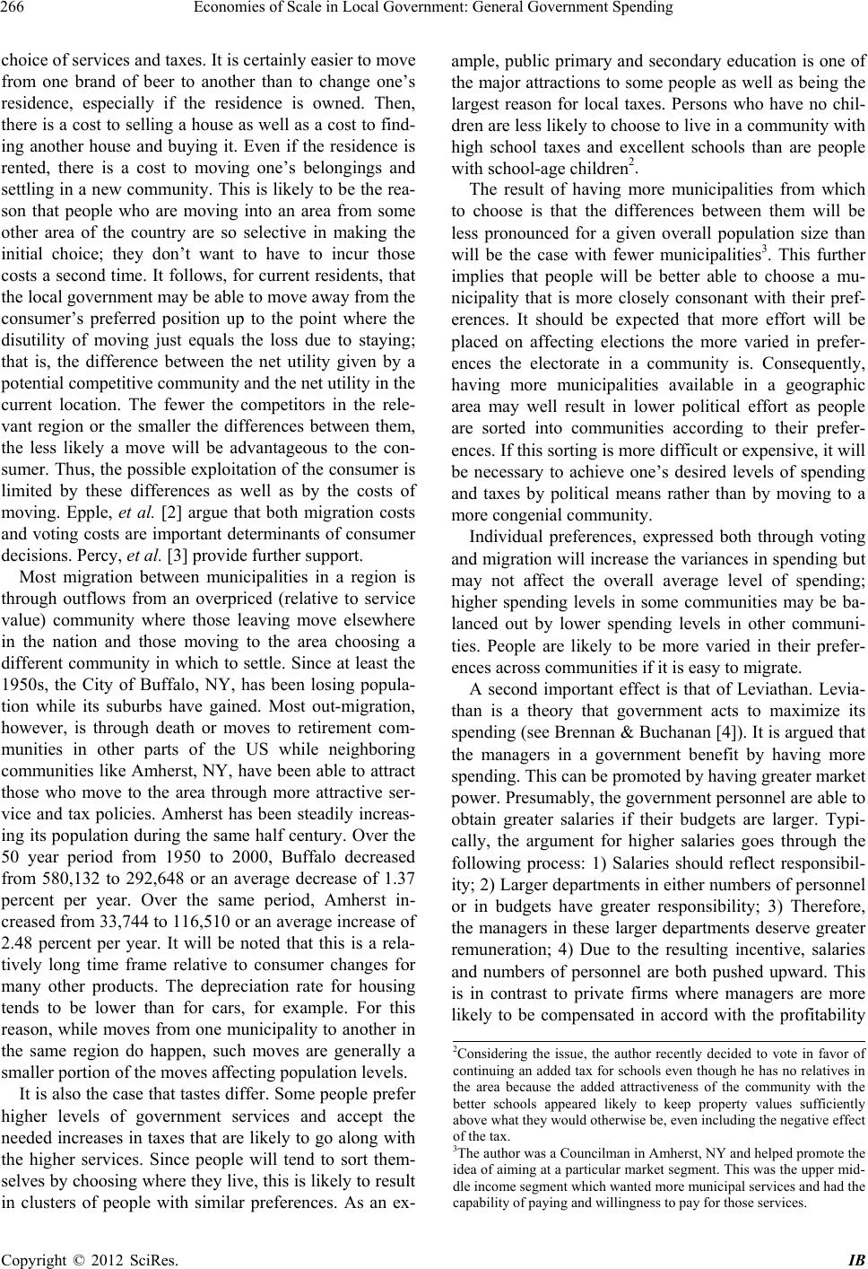

Economies of Scale in Local Government: General Government Spending
266
choice of services and taxes. It is certainly easier to move
from one brand of beer to another than to change one’s
residence, especially if the residence is owned. Then,
there is a cost to selling a house as well as a cost to find-
ing another house and buying it. Even if the residence is
rented, there is a cost to moving one’s belongings and
settling in a new community. This is likely to be the rea-
son that people who are moving into an area from some
other area of the country are so selective in making the
initial choice; they don’t want to have to incur those
costs a second time. It follows, for current residents, that
the local government may be able to move away from the
consumer’s preferred position up to the point where the
disutility of moving just equals the loss due to staying;
that is, the difference between the net utility given by a
potential competitive community and the net utility in the
current location. The fewer the competitors in the rele-
vant region or the smaller the differences between them,
the less likely a move will be advantageous to the con-
sumer. Thus, the possible exploitation of the consumer is
limited by these differences as well as by the costs of
moving. Epple, et al. [2] argue that both migration costs
and voting costs are important determinants of consumer
decisions. Percy, et al. [3] provide further support.
Most migration between municipalities in a region is
through outflows from an overpriced (relative to service
value) community where those leaving move elsewhere
in the nation and those moving to the area choosing a
different community in which to settle. Since at least the
1950s, the City of Buffalo, NY, has been losing popula-
tion while its suburbs have gained. Most out-migration,
however, is through death or moves to retirement com-
munities in other parts of the US while neighboring
communities like Amherst, NY, have been able to attract
those who move to the area through more attractive ser-
vice and tax policies. Amherst has been steadily increas-
ing its population during the same half century. Over the
50 year period from 1950 to 2000, Buffalo decreased
from 580,132 to 292,648 or an average decrease of 1.37
percent per year. Over the same period, Amherst in-
creased from 33,744 to 116,510 or an average increase of
2.48 percent per year. It will be noted that this is a rela-
tively long time frame relative to consumer changes for
many other products. The depreciation rate for housing
tends to be lower than for cars, for example. For this
reason, while moves from one municipality to another in
the same region do happen, such moves are generally a
smaller portion of the moves affecting population levels.
It is also the case that tastes differ. Some people prefer
higher levels of government services and accept the
needed increases in taxes that are likely to go along with
the higher services. Since people will tend to sort them-
selves by choosing where they live, this is likely to result
in clusters of people with similar preferences. As an ex-
ample, public primary and secondary education is one of
the major attractions to some people as well as being the
largest reason for local taxes. Persons who have no chil-
dren are less likely to choose to live in a community with
high school taxes and excellent schools than are people
with school-age children2.
The result of having more municipalities from which
to choose is that the differences between them will be
less pronounced for a given overall population size than
will be the case with fewer municipalities3. This further
implies that people will be better able to choose a mu-
nicipality that is more closely consonant with their pref-
erences. It should be expected that more effort will be
placed on affecting elections the more varied in prefer-
ences the electorate in a community is. Consequently,
having more municipalities available in a geographic
area may well result in lower political effort as people
are sorted into communities according to their prefer-
ences. If this sorting is more difficult or expensive, it will
be necessary to achieve one’s desired levels of spending
and taxes by political means rather than by moving to a
more congenial community.
Individual preferences, expressed both through voting
and migration will increase the variances in spending but
may not affect the overall average level of spending;
higher spending levels in some communities may be ba-
lanced out by lower spending levels in other communi-
ties. People are likely to be more varied in their prefer-
ences across communities if it is easy to migrate.
A second important effect is that of Leviathan. Levia-
than is a theory that government acts to maximize its
spending (see Brennan & Buchanan [4]). It is argued that
the managers in a government benefit by having more
spending. This can be promoted by having greater market
power. Presumably, the government personnel are able to
obtain greater salaries if their budgets are larger. Typi-
cally, the argument for higher salaries goes through the
following process: 1) Salaries should reflect responsibil-
ity; 2) Larger departments in either numbers of personnel
or in budgets have greater responsibility; 3) Therefore,
the managers in these larger departments deserve greater
remuneration; 4) Due to the resulting incentive, salaries
and numbers of personnel are both pushed upward. This
is in contrast to private firms where managers are more
likely to be compensated in accord with the profitability
2Considering the issue, the author recently decided to vote in favor o
f
continuing an added tax for schools even though he has no relatives in
the area because the added attractiveness of the community with the
better schools appeared likely to keep property values sufficiently
above what they would otherwise be, even including the negative effect
of the tax.
3The author was a Councilman in Amherst, NY and helped promote the
idea of aiming at a particular market segment. This was the upper mid-
dle income segment which wanted more municipal services and had the
capability of paying and willingness to pay for those services.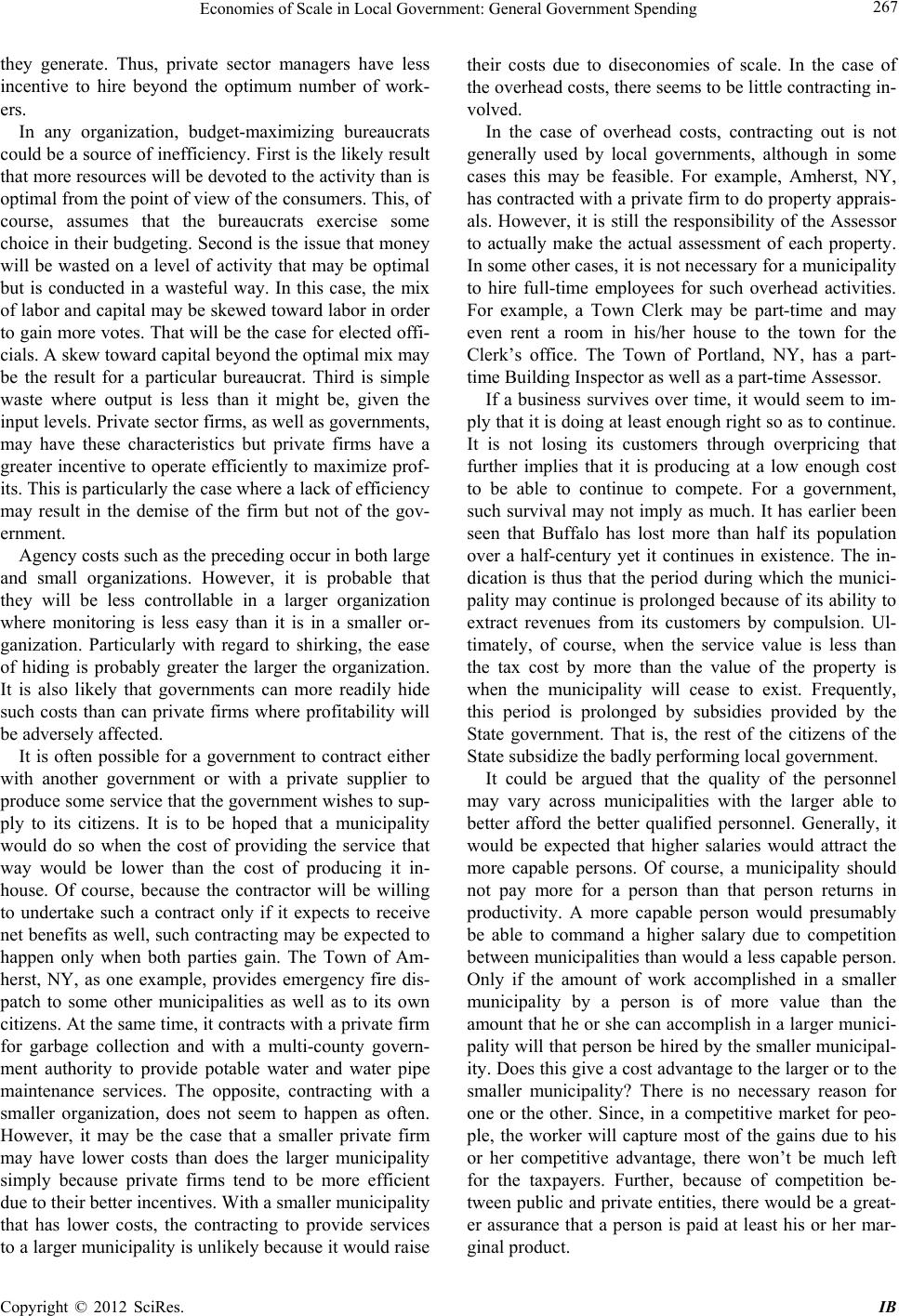

Economies of Scale in Local Government: General Government Spending 267
they generate. Thus, private sector managers have less
incentive to hire beyond the optimum number of work-
ers.
In any organization, budget-maximizing bureaucrats
could be a source of inefficiency. First is the likely result
that more resources will be devoted to the activity than is
optimal from the point of view of the consumers. This, of
course, assumes that the bureaucrats exercise some
choice in their budgeting. Second is the issue that money
will be wasted on a level of activity that may be optimal
but is conducted in a wasteful way. In this case, the mix
of labor and capital may be skewed toward labor in order
to gain more votes. That will be the case for elected offi-
cials. A skew toward capital beyond the optimal mix may
be the result for a particular bureaucrat. Third is simple
waste where output is less than it might be, given the
input levels. Private sector firms, as well as governments,
may have these characteristics but private firms have a
greater incentive to operate efficiently to maximize prof-
its. This is particularly the case where a lack of efficiency
may result in the demise of the firm but not of the gov-
ernment.
Agency costs such as the preceding occur in both large
and small organizations. However, it is probable that
they will be less controllable in a larger organization
where monitoring is less easy than it is in a smaller or-
ganization. Particularly with regard to shirking, the ease
of hiding is probably greater the larger the organization.
It is also likely that governments can more readily hide
such costs than can private firms where profitability will
be adversely affected.
It is often possible for a government to contract either
with another government or with a private supplier to
produce some service that the government wishes to sup-
ply to its citizens. It is to be hoped that a municipality
would do so when the cost of providing the service that
way would be lower than the cost of producing it in-
house. Of course, because the contractor will be willing
to undertake such a contract only if it expects to receive
net benefits as well, such contracting may be expected to
happen only when both parties gain. The Town of Am-
herst, NY, as one example, provides emergency fire dis-
patch to some other municipalities as well as to its own
citizens. At the same time, it contracts with a private firm
for garbage collection and with a multi-county govern-
ment authority to provide potable water and water pipe
maintenance services. The opposite, contracting with a
smaller organization, does not seem to happen as often.
However, it may be the case that a smaller private firm
may have lower costs than does the larger municipality
simply because private firms tend to be more efficient
due to their better incentives. With a smaller municipality
that has lower costs, the contracting to provide services
to a larger municipality is unlikely because it would raise
their costs due to diseconomies of scale. In the case of
the overhead costs, there seems to be little contracting in-
volved.
In the case of overhead costs, contracting out is not
generally used by local governments, although in some
cases this may be feasible. For example, Amherst, NY,
has contracted with a private firm to do property apprais-
als. However, it is still the responsibility of the Assessor
to actually make the actual assessment of each property.
In some other cases, it is not necessary for a municipality
to hire full-time employees for such overhead activities.
For example, a Town Clerk may be part-time and may
even rent a room in his/her house to the town for the
Clerk’s office. The Town of Portland, NY, has a part-
time Building Inspector as well as a part-time Assessor.
If a business survives over time, it would seem to im-
ply that it is doing at least enough right so as to continue.
It is not losing its customers through overpricing that
further implies that it is producing at a low enough cost
to be able to continue to compete. For a government,
such survival may not imply as much. It has earlier been
seen that Buffalo has lost more than half its population
over a half-century yet it continues in existence. The in-
dication is thus that the period during which the munici-
pality may continue is prolonged because of its ability to
extract revenues from its customers by compulsion. Ul-
timately, of course, when the service value is less than
the tax cost by more than the value of the property is
when the municipality will cease to exist. Frequently,
this period is prolonged by subsidies provided by the
State government. That is, the rest of the citizens of the
State subsidize the badly performing local government.
It could be argued that the quality of the personnel
may vary across municipalities with the larger able to
better afford the better qualified personnel. Generally, it
would be expected that higher salaries would attract the
more capable persons. Of course, a municipality should
not pay more for a person than that person returns in
productivity. A more capable person would presumably
be able to command a higher salary due to competition
between municipalities than would a less capable person.
Only if the amount of work accomplished in a smaller
municipality by a person is of more value than the
amount that he or she can accomplish in a larger munici-
pality will that person be hired by the smaller municipal-
ity. Does this give a cost advantage to the larger or to the
smaller municipality? There is no necessary reason for
one or the other. Since, in a competitive market for peo-
ple, the worker will capture most of the gains due to his
or her competitive advantage, there won’t be much left
for the taxpayers. Further, because of competition be-
tween public and private entities, there would be a great-
er assurance that a person is paid at least his or her mar-
ginal product.

Economies of Scale in Local Government: General Government Spending
268
However, it may be that reducing the number of possi-
ble competitors by mergers will allow municipalities to
obtain monopsony gains in hiring. Since, for the best
people, the relevant market is likely to be more than local,
perhaps even national, that argument is unlikely to have
validity. In addition, the gains to the very well qualified
people who may have monopoly gains through fewer
competitors may more than offset any monopsony gains.
Possibly, the gains available through the monopoly pow-
er will attract better people who will then share the bene-
fits of their abilities with the customers/taxpayers, par-
tially offsetting the losses due to the market power. It is
an empirical question as to how this effect, if it exists,
may work out in practice.
The original location of a city was usually determined
because it had location related advantages over alterna-
tive sites. Because it typically still has those advantages,
it should be able to compete well with any surrounding
communities4. However, if it is exploiting those resulting
monopoly rents for the advantage of the government
functionaries, it may be advantageous for a new city to
start up in competition. The customers will then gain the
benefits of that competition5.
The issue of whether the suburbs harm the city is
sometimes raised from the point of view that it takes re-
sources away from the city and thus makes the city worse
off. Hawkins and Ihrke [5] reviewed numerous studies on
this. A preponderance of these found either that there
was no effect or that fragmentation decreased costs. Of
course, the resources under consideration belong to the
consumers, not to the city. The argument, in effect, is the
same as that the Berlin Wall which prevented people
leaving was useful because the people belonged to East
Germany. Staley [6] argues that the cities actually exploit
the suburbs. A simple analysis shows that, because resi-
dences do not pay their full costs in taxes while busi-
nesses and industries pay more than their full costs, sub-
urbs which are primarily residential take more of the cost
burden while leaving cities with more of the tax base.
Filer and Kenny [7] find that city/county consolidation is
primarily a way for the poorer city residents to exploit
wealthier suburbanites.
The next argument, also much used, is that there are
economies of scale. This, often without empirical evi-
dence that there are such economies, is asserted to re-
quire that mergers of municipalities take place in order to
save the taxpayers money. This is the issue to be studied
in this paper. In many cases, if such economies existed,
they could be achieved by contracting out the function
either to private industry or to another government. The
“Lakewood Plan” is such intergovernmental contracting
where Lakewood CA chose to actually produce almost
no services while still providing them (see Ostrom, Tie-
bout and Warren [8] for a discussion of this). Why the
elected officials would not choose to do such contracting
if it were that beneficial is not generally asked. It is sim-
ply asserted as a reason that the local officials would lose
power and perks.
On the other side of the issue is the argument that
mergers would result in fewer choices on the level of
services for the consumers. Nelson [9] argues that con-
sumers prefer more choice. Falcone and Lan [10] argue
that the more local the government, the better it knows
the consumers’ preferences and the better it can adjust to
local conditions. Olson [11] also argues for variations in
services. The author, while in local elective office, made
successful efforts for his local government to aim for a
specific market segment, adjusting the levels of services
and the consequent taxes to appeal to that particular
market. There is a loss accruing to consumers who have
heterogeneous preferences when they are forced into a
common mold (Procrustes was not a good guy.) The
magnitude of this loss in the case of metropolitanization
will depend on the degree of these differences in prefer-
ence.
Another argument against metropolitanization is that
the governments will be able to exploit their increased
market power to extract gains from the taxpayers. Lynk
[12] as well as Vita and Sacher [13] find that mergers of
hospitals result in price increases. Abelson [14] and Di-
Lorenzo [15] argue for this exploitation hypothesis. Kne-
ebone [16] finds that decentralization would reduce costs.
Wagner and Weber [17] also find that governments,
when able, act as monopolists. To date, however, the em-
pirical work has been spotty in this area. Again, this issue
will be explored in this paper.
4Buffalo, NY, has lost its port advantage because of the construction o
f
the St. Lawrence Seaway in Canada that allows ships to bypass (and
eliminates offloading in) Buffalo. However, it still retains the advan-
tages of higher ground, existing infrastructure, and access to the water-
front. It ought to be able to compete well with suburbs that are located
in swamps or in places where it is otherwise difficult to build.
5There are also some other arguments made as to why local govern-
ments should be merged. One is the purported existence of externalities
If the smoke from a factory in one municipality blows into a neighbor-
ing municipality, the latter suffers uncompensated harm. Shoup [42]
made essentially this argument. However, it isn’t the municipality that
is harmed but the property owner receiving the smoke. If both the
emitter of smoke and the receiver of it are in the same municipality,
there is no reason to believe that the decision made by that municipality
will be any better than the decision made between the two municipali-
ties. If the property rights are well-defined and are enforced, bargaining
can take place and will yield the optimal result as per Coase [43].
Numerous papers have been written in regard to whe-
ther there are or are not economies of scale in local gov-
ernment. The first issue was whether large cities spend
more or less per capita than smaller cities. Gabler [18],
Zax [19] and Joulfaian and Marlow [20] found that they
spend more. Deller [21] reviewed several studies that
found that costs increased after consolidation. Rodden
[22] found that decentralization decreased costs. Couch,

Economies of Scale in Local Government: General Government Spending 269
et al. [23] found for several government activities that
there are diseconomies of scale.
What about diseconomies of scale? Brempong [24]
and Gyapong and Brempong [25] found diseconomies of
scale in policing. Ostrom and Whittaker [26] found less
satisfaction with police in larger cities. Sjoquist and
Walker [27] found economies of scale in property as-
sessment. Brynes and Dollery [28] review a number of
studies and find that there is no evidence of economies of
scale.
The next issue was efficiency; residents of larger cities
might simply have a preference for a higher level of ser-
vices to account for their higher spending. Are larger
cities more efficient? Hirsch [29] did not find that con-
solidation increased efficiency. Lockwood [30] finds de-
centralized government to be more efficient. Oliver [31]
finds that citizens monitor larger governments less which
could lead to less efficiency. Bardhan [32] also found
that devolution of services to local governments resulted
in greater efficiency.
There are also a number of papers that find U shaped
average cost curves. This implies that there is an optimal
size for governments. Loehman and Emerson [33], Sha-
piro [34] Drake and Simper [35], and Southwick [36] all
effectively find such cost curves. This implies econo-
mies of scale for smaller municipalities and disecono-
mies for larger municipalities. Most past studies assumed
that there were either economies or diseconomies over
the entire range and used empirical methods that did not
allow for the finding of a U shaped cost curve.
3. The Study Design
This study will explicitly allow for economies of scale,
diseconomies of scale, and a possible U shaped average
cost curve. Another important issue to be explicitly con-
sidered is whether local governments actually are able to
use any market power they may have to exploit their cus-
tomers. Both of these issues remain controversial and
need careful empirical work.
The study, as stated above, will focus on overhead
costs. These overhead costs, which are also referred to as
general government costs, include all costs of the local
government less the following:
 Education
 Police
 Fire
 Other public safety
 Health
 Transportation (highways and mass transit, generally)
 Economic assistance (public welfare payments)
 Culture & recreation
 Utilities (sewers, drainage, water)
 Other home & community services
Each of these excluded costs has more choice embed-
ded in it than do the overhead costs. Consequently, it
would be necessary to include the amounts (quantities
per capita) of those services as well as their costs in
terms of the local decisions made.
There is much less choice involved in the area of the
overhead items. Therefore, there tends to be much less
variation in the level of services provided across munici-
palities. Major components of these costs include:
 Assessment/tax collection
 Zoning/planning
 Building code enforcement
 Legal
 Clerical
 Legislative/executive
 Financial/fiscal management
In regard to these particular services, it will be pre-
sumed that the residents desire mainly to achieve the
lowest feasible cost. Because the quality does not differ
appreciably (except in the minds of the providers), the
lowest cost delivers the lowest tax effects and therefore
the highest utility. Of course, if mistakes or errors are
made by the providers, that may result in citizen dis-
pleasure. However, that is much less likely for these ac-
tivities than is concern over the services (excluded here)
that provide direct utility to the users/citizenry.
It is true, of course, that decisions made by the legisla-
tive body may not be optimal according to some of the
citizenry. However, the issue there is not generally the
cost but rather the choices made by the elected officials.
For example, the legislators may approve of some re-
zoning which is opposed by some of the people. While
some of the citizens would like to replace some of the
elected officials after such decisions, typically decisions
are made by the elected officials with the idea in mind of
maximizing the proportion of the voters who will ap-
prove the decision6. Overhead costs and the associated
costs are generally desired to be minimized since there is
no constituency for increasing them as there is for rec-
reational service, for example.
It will be supposed that there is an average cost per
capita, AC, function for the overhead services that in-
cludes the population of the municipality and the market
power of the government of the municipality. Let that
function be:


ACfPop, HH, X (1)
where Pop is the population, HH is a measure of the
market power, and X is other variables. The first deriva-
tive with respect to population of the function chosen
should have the capability of being of one sign at one
6In politics, of course, “friends come and go while enemies accumu-
late”. Thus, even accuracy in choosing decisions according to pleasing
the electorate may result in eventually losing elections.

Economies of Scale in Local Government: General Government Spending
270
population level and of another sign at another popula-
tion level. Two functions that have this capability are:

ACabPopc1 PopdHHeX (2)
 

ln ACab*ln Popc*ln Popln Pop
d*ln HHe*HH
 
 (3)
The derivative of Equation (2) with respect to Pop is;

2
ACPopbc1 Pop

(2a)
If Pop is large, the value of the derivative approaches b,
which can be either positive or negative, implying either
diseconomies or economies of scale, respectively. At a
lower value of Pop, the value approaches b – c, which
will be positive if b > 0 and c < 0 and will be negative if
b < 0 and c > 0. If b and c are both positive or are both
negative, the issue of economies or diseconomies will
depend on the relative absolute magnitudes. Thus, a vari-
ety of alternatives can be accommodated.
Suppose that both b and c are positive in Equation (2).
Then, there exists an optimum population size to mini-
mize AC. That population is:

0.5
Popcb (2b)
With the translog function, Equation (3), the derivative
with respect to Pop is:

ACPopb2clnPopPop 
 
(3a)
If b > 0 and c > 0, the result is diseconomies of scale
and, if b < 0 and c < 0, the result is economies of scale.
At relatively (compared to b/c) small values for Pop,
diseconomies result from b > 0 and economies result
from b < 0. At large values for Pop relative to b/c, dis-
economies result from c > 0 and economies result from c <
0. Again, a variety of alternative outcomes can be accom-
modated.
Suppose that Equation (3) is estimated and that b < 0
while c > 0. Then the optimal population (minimum AC)
becomes;

Popexpb 2c

(3b)
Now for the variables denoted as X. One is a dummy
variable for City. In New York State, Towns and Cities
have mutually exclusive territories and, in the aggregate,
include all lands in the state. Cities have different laws
applicable to them than do Towns; thus, the variable to
control for that difference. One interesting difference
might be the proportion of power vested in district coun-
cilmen that is generally higher in cities since most coun-
cilmen are elected at-large in towns7.
Another issue is presented by the various years. The
data are for a number of years. They are adjusted for
Consumer Price Index (CPI) levels for the various years
to be in 2004 dollars. Nonetheless, there may be other
differences to be accounted for over the different years.
Thus, dummy variables for the years may need to be in-
cluded to account for these differences8.
4. Data
The towns and cities in New York State will comprise
the data set. The governments involved are the truly local
governments, towns and cities9. If one lives in New York
State, one lives in either a city or in a town. New York
City will be left out of the data set because it is so sub-
stantially different as would skew any results10. The rea-
son for using a single state is to ensure that all of the mu-
nicipalities operate under a single legal system and state-
imposed set of constraints. Each observation is for a sin-
gle town or city in a particular year11. As an example of
how the set is consistent is that New York State allows
(essentially requires) all the municipalities to have their
employees be represented by unions. How they deal with
the unions is then controlled by State regulations that are
relatively uniform across the state.
There are approximately 932 towns and 61 cities in
New York outside of New York City. This includes all of
the land area of the state, again not including New York
City. This follows from the design of the governments in
New York where every parcel of land is in either a city
or a town. There are also villages, but these are each in-
cluded in one or more towns and therefore are not truly
separate governments12.
The years for which these data are readily available
include 1977 through 2004. The source is various (on-
line) years of “Financial Data for Local Governments”
from the New York State Comptroller’s Office. Because
the original source is reports from the Towns and Cities
themselves, there are occasional missing data where a
municipality was late in reporting or did not report. Po-
tentially, there may be up to 26,811 observations. In
practice, because of missing observations and missing
8The values for these estimated coefficients will not be reported since
they are not of interest here.
9In New York State, as in most northern and eastern states, townships
(towns) are the most local municipalities while in the western and
southern states, the county is the most local.
10Over 42 percent of the population of New York State resided in New
York City in 2004 (see US Statistical Abstract 2006, p.21 and p.34).
Further, the total spending per capita in NYC in 2004 was over $7900
while for the rest of the local governments, the total spending per cap-
ita was just under $4,000 or about half as much.
11There are also villages in New York. These overlap or are included in
towns. Generally, they provide services not provided or provided at a
lower level by the overlapping town(s).
12It might even be argued that homeowners’ associations act as gov-
ernments, providing services and levying taxes (fees) on members.
7It has been shown by Southwick [41] that greater power for ward
councilmen results in higher spending levels.

Economies of Scale in Local Government: General Government Spending 271
items in some reports, there are fewer13. New York City,
as noted above, is not included in the data set.
The population figures are only available accurately
for the census reports every 10 years. In order to compute
the population figures for each community in the other
years, it was necessary to interpolate between the census
figures. For the years after the 2000 census, the popula-
tion for each community was computed using the as-
sumption that it had continued to change at the same an-
nual amount it had changed from 1990 to 2000.
Market power is defined as the Herfindahl-Hirschman
(HH) Index with the county as the market area. The
population in each Town and City in that county as a pro-
portion of the total county population is squared and
multiplied by 10,000 to give the HH value for that mu-
nicipality. The total of these HH values across the Towns
and Cities in that county gives the relevant HH number
for the county and measures the market power for the
communities in that county. It is thus assumed that peo-
ple have a choice of communities only within their coun-
ty14.
All the financial data were adjusted by the CPI to 2004
values. Thus, the per capita financial values were ad-
justed as well.
The characteristics of each of these variables are given
in Table 1.
The dependent variable, either LNRGP or RGGPOP,
has the fewest observations and so will determine the
number of observations used in the regressions.
The largest city (not including NYC) in the census of
2000 was Buffalo with 292,648 people and the largest
town was Hempstead with 755,924. The smallest city
was Sherrill with 3147 and the smallest town was Red
House with 38. The median city was Plattsburgh with
18,816 and the median town was between Caroline at
2910 and Pamelia at 2897. The average city size in 2000
was 37,146 and the average town was 9326.
Table 2 gives the correlations among the variables
used.
The only substantial concern is the high correlation be-
tween LNPOP and LNPLNP since both are to be used as
independent variables in a regression. However, with
POP and POP1 essentially uncorrelated in the corre-
sponding quadratic (non-translog) regression, this con-
cern should be alleviated. Further, correlation among in-
dependent variables has the effect of increasing the stan-
dard errors and so should only have the effect of reduc-
ing the likelihood of finding the effect which is looked
for. Also, note that the correlation between City and Pop
is only 0.18 so the larger population municipalities are
not necessarily cities.
Note that the HH Index is not highly correlated with
municipality size. This suggests that a higher population
for one municipality generally tends to show up with
other municipalities in the county also having higher po-
pulations15. That would be consistent with municipali-
ties responding to market forces by seeking market ni-
ches within their counties.
5. Results
The following three Tables 3(a)-(c), are the results of the
regressions using the Average Cost per Capita of the lo-
cal governments over the 28-year time period as the de-
pendent variable. As noted earlier, all of the financial
variables have been adjusted by the CPI to 2004 dollars.
Table 3(a) is OLS, Table 3(b) uses Year dummies (the
coefficients of which are not reported), and Table 3(c)
computes a frontier result16. These are all done using
LIMDEP [37].
Also included at the bottom of each table is the im-
plied population for the lowest average cost municipality
for that regression, where such a computation is possible.
The number of observations with complete data in
each of the above regressions is 27,509. Thus, there is a
large number for degrees of freedom in each case. The
very substantial t-statistics that show that each of the
variables is highly significant in each equation is partly
the result of the large number of observations.
Still, the significance of the results tends to lead to the
conclusion that these equations truly are meaningful in
the attempt to explain the variation in the average cost
data. Further, the average cost regressions do appear to
explain a substantial part of that variation. The estimated
lowest cost populations appear to be somewhere between
17,000 and 21,000.
The frontier regressions are interesting because, unlike
the other regressions, they are estimates of the minimum
possible costs. The fact that each of the coefficients in
these regressions is significant gives a good deal of con-
fidence in the results. Further, the result that the mini-
mum cost population estimates are very like the other
minimum cost population estimates from the OLS and
panel regressions gives more support to the U-shape of
the cost function and the level of the true optimum popu-
lation.
13There are also fewer observations because there were only 930 Towns
at the beginning of the period while there were 932 at the end of the
p
eriod.
14Of course, some people do commute across county lines. In a similar
fashion, some people buy office supplies from other than the big three
b
ox stores, Office Max, Office Depot, and Staples. However, as a
boundary must be set somewhere, as the FTC did with the big three, so
this paper will use the county which had its boundaries set for effi-
ciency some time ago.
It can be inferred with some confidence that very small
15The correlation between the population of the county and the HH
Index is 0.4.
16The distribution is assumed to be half-normal.

Economies of Scale in Local Government: General Government Spending
272
Table 1. Variable characteristics.
Name Variable Mean Std. Dev. Minimum Maximum Cases
Pop Population 10,795 37,096 1 768,052 27775
Pop1 1/Population 6.11E−04 7.05E−03 1.30E−06 1 27775
HH HH Index 1214.8 580.0 565.2 3986.6 27799
RGGPop Real Gen. Gov. Exp/Pop 99.13 101.14 13.70 2,475.97 27509
LnRGP ln(RGGPOp) 4.3610 0.6170 2.6171 7.8144 27509
LnPop ln(POp) 8.2030 1.2728 0 13.5516 27775
LnPLNP ln(POp)*ln(POp) 68.9088 21.9661 0 183.6462 27775
LNH ln(HH) 7.0078 0.4206 6.3372 8.2907 27799
Year Year 1990.5 8.1 1977.0 2004.0 27799
CPI CPI 130.23 36.99 60.60 188.90 27799
City City = 1, Town = 0 6.14E−02 0.2401 0 1 27799
Table 2. Correlations among variables.
Pop Pop1 HH RGGPopLnRGP LnPop LnPLNP LNH
Pop 1.00 −0.13 0.32 0.05 0.08 0.56 0.63 0.25
Pop1 −0.13 1.00 −0.10 0.43 0.32 −0.58 −0.51 −0.09
HH 0.32 −0.10 1.00 0.04 0.05 0.30 0.32 0.97
RGGPop 0.05 0.43 0.04 1.00 0.84 −0.13 −0.08 0.04
LnRGP 0.08 0.32 0.05 0.84 1.00 −0.08 −0.03 0.04
LnPop 0.56 −0.58 0.30 −0.13 −0.08 1.00 0.99 0.26
LnPLNP 0.63 −0.51 0.32 −0.08 −0.03 0.99 1.00 0.28
LNH 0.25 −0.09 0.97 0.04 0.04 0.26 0.28 1.00
Year 0.01 −0.04 −0.06 0.14 0.22 0.05 0.05 −0.08
CPI 0.02 −0.04 −0.06 0.14 0.22 0.05 0.05 −0.07
City 0.18 −0.12 0.05 0.21 0.31 0.36 0.37 0.04
communities have higher average costs because of their
size and that larger communities have higher average
costs because of their size. While the mean population is
only about half the optimal size for this function, advo-
cacy of mergers for many communities is not necessarily
warranted17.
Next, the results for the estimated translog cost func-
tions are reported in Tables 4(a)-(c). These are the OLS,
panel with dummies for the years, and frontier regres-
sions as above.
The number of complete observations is 27,509. All of
the estimated coefficients are highly significant, except
for the ln(HH Index) in Tables 4(a) and (c) where City is
not included. The optimal population here is found to be
somewhere between 6300 and 11,000. In every one of
the above 27 regressions, the result is a U-shaped curve,
implying that there exists an optimal sized population to
minimize the average per capita cost.
It can also be concluded that greater market power
does result in higher costs, thus suggesting that local
governments do seek to exploit their market power to
extract rents from the public. Mergers that would in-
crease such market power would result in increased ex-
ploitation even if the resulting population were to remain
near the optimal. Further, the results show that the market power, as
measured by the county HH Index, is a significant factor
increasing the average cost. Apparently the market power
17Optimal populations for other municipal functions would also be
relevant.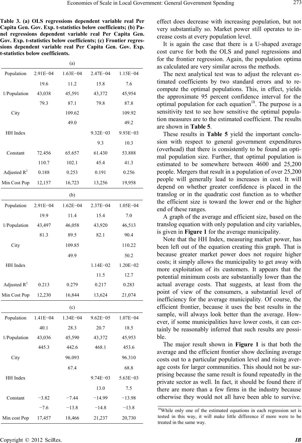

Economies of Scale in Local Government: General Government Spending 273
Table 3. (a) OLS regressions dependent variable real Per
Capita Gen. Gov. Exp. t-statistics below coefficients; (b) Pa-
nel regressions dependent variable real Per Capita Gen.
Gov. Exp. t-statistics below coefficients; (c) Frontier regres-
sions dependent variable real Per Capita Gen. Gov. Exp.
t-statistics below coefficien ts .
(a)
Population 2.91E−04 1.63E−04 2.47E−04 1.15E−04
19.6 11.2 15.8 7.6
1/Population 43,038 45,591 43,372 45,954
79.3 87.1 79.8 87.8
City 109.62 109.92
49.0 49.2
HH Index 9.32E−03 9.93E−03
9.3 10.3
Constant 72.456 65.657 61.430 53.888
110.7 102.1 45.4 41.3
Adjusted R2 0.188 0.253 0.191 0.256
Min Cost Pop 12,157 16,723 13,256 19,958
(b)
Population 2.91E−04 1.62E−04 2.37E−04 1.05E−04
19.9 11.4 15.4 7.0
1/Population 43,497 46,058 43,920 46,513
81.3 89.5 82.1 90.4
City 109.85 110.22
49.9 50.2
HH Index 1.14E−02 1.20E−02
11.5 12.7
Adjusted R2 0.213 0.279 0.217 0.283
Min Cost Pop 12,230 16,844 13,624 21,074
(c)
Population 1.41E−04 1.34E−04 9.62E−05 1.07E−04
40.1 28.3 20.7 18.5
1/Population 43,036 45,590 43,372 45,953
445.3 442.6 468.1 453.6
City 96.093 96.310
67.4 68.8
HH Index 9.74E−03 5.63E−03
13.0 7.5
Constant −3.82 −7.44 −14.99 −13.98
−7.6 −13.8 −14.8 −13.8
Min cost Pop 17,457 18,466 21,237 20,730
effect does decrease with increasing population, but not
very substantially so. Market power still operates to in-
crease costs at every population level.
It is again the case that there is a U-shaped average
cost curve for both the OLS and panel regressions and
for the frontier regression. Again, the population optima
as calculated are very similar across the methods.
The next analytical test was to adjust the relevant es-
timated coefficients by two standard errors and to re-
compute the optimal populations. This, in effect, yields
the approximate 95 percent confidence interval for the
optimal population for each equation18. The purpose is a
sensitivity test to see how sensitive the optimal popula-
tion measures are to the estimated coefficient. The results
are shown in Table 5.
These results in Table 5 yield the important conclu-
sion with respect to general government expenditures
(overhead) that there is consistently to be found an opti-
mal population size. Further, that optimal population is
estimated to be somewhere between 4600 and 25,200
people. Mergers that result in a population of over 25,200
people will generally lead to increases in cost. It will
depend on whether greater confidence is placed in the
translog or in the quadratic cost function as to whether
the efficient size is toward the lower end or the higher
end of these ranges.
A graph of the average and efficient size, based on the
translog equation with only population and city variables,
is given in Figure 1 for the average municipality.
Note that the HH Index, measuring market power, has
been left out of the equation creating this graph. That is
because greater market power does not require higher
costs; it simply allows the municipality to get away with
more exploitation of its customers. It appears that the
potential minimum costs are substantially lower than the
actual average costs. That suggests, at least from the
point of view of the consumers, a substantial level of
inefficiency for the average municipality. Of course, the
efficient frontier, because it uses the best results in the
sample, will always look better than the average. How-
ever, if some municipalities have lower costs, it can cer-
tainly be reasonably inferred that such results are possi-
ble.
The major result shown in Figure 1 is that both the
average and the efficient frontier show declining average
costs out to a particular population level and rising aver-
age costs for larger communities. This should not be sur-
prising because the same result is found repeatedly in the
private sector as well. In fact, it should be found there if
there are more than a few firms in the industry because
otherwise they would not all have been able to survive.
18While only one of the estimated equations in each regression set is
tested in this way, it will make little difference if more were to be
treated in the same way.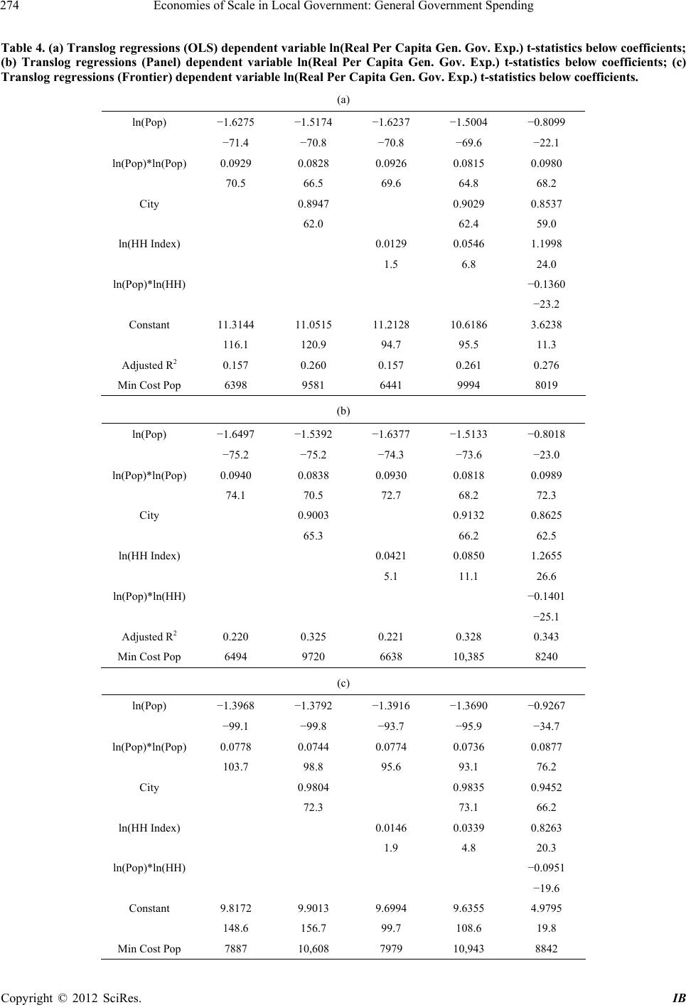

Economies of Scale in Local Government: General Government Spending
274
Table 4. (a) Translog regressions (OLS) dependent variable ln(Real Per Capita Gen. Gov. Exp.) t-statistics below coefficients;
(b) Translog regressions (Panel) dependent variable ln(Real Per Capita Gen. Gov. Exp.) t-statistics below coefficients; (c)
Translog regressions (Frontier) dependent variable ln(Real Per Capita Gen. Gov. Exp.) t-statistics below coefficients.
(a)
ln(Pop) −1.6275 −1.5174 −1.6237 −1.5004 −0.8099
−71.4 −70.8 −70.8 −69.6 −22.1
ln(Pop)*ln(Pop) 0.0929 0.0828 0.0926 0.0815 0.0980
70.5 66.5 69.6 64.8 68.2
City 0.8947 0.9029 0.8537
62.0 62.4 59.0
ln(HH Index) 0.0129 0.0546 1.1998
1.5 6.8 24.0
ln(Pop)*ln(HH) −0.1360
−23.2
Constant 11.3144 11.0515 11.2128 10.6186 3.6238
116.1 120.9 94.7 95.5 11.3
Adjusted R2 0.157 0.260 0.157 0.261 0.276
Min Cost Pop 6398 9581 6441 9994 8019
(b)
ln(Pop) −1.6497 −1.5392 −1.6377 −1.5133 −0.8018
−75.2 −75.2 −74.3 −73.6 −23.0
ln(Pop)*ln(Pop) 0.0940 0.0838 0.0930 0.0818 0.0989
74.1 70.5 72.7 68.2 72.3
City 0.9003 0.9132 0.8625
65.3 66.2 62.5
ln(HH Index) 0.0421 0.0850 1.2655
5.1 11.1 26.6
ln(Pop)*ln(HH) −0.1401
−25.1
Adjusted R2 0.220 0.325 0.221 0.328 0.343
Min Cost Pop 6494 9720 6638 10,385 8240
(c)
ln(Pop) −1.3968 −1.3792 −1.3916 −1.3690 −0.9267
−99.1 −99.8 −93.7 −95.9 −34.7
ln(Pop)*ln(Pop) 0.0778 0.0744 0.0774 0.0736 0.0877
103.7 98.8 95.6 93.1 76.2
City 0.9804 0.9835 0.9452
72.3 73.1 66.2
ln(HH Index) 0.0146 0.0339 0.8263
1.9 4.8 20.3
ln(Pop)*ln(HH) −0.0951
−19.6
Constant 9.8172 9.9013 9.6994 9.6355 4.9795
148.6 156.7 99.7 108.6 19.8
Min Cost Pop 7887 10,608 7979 10,943 8842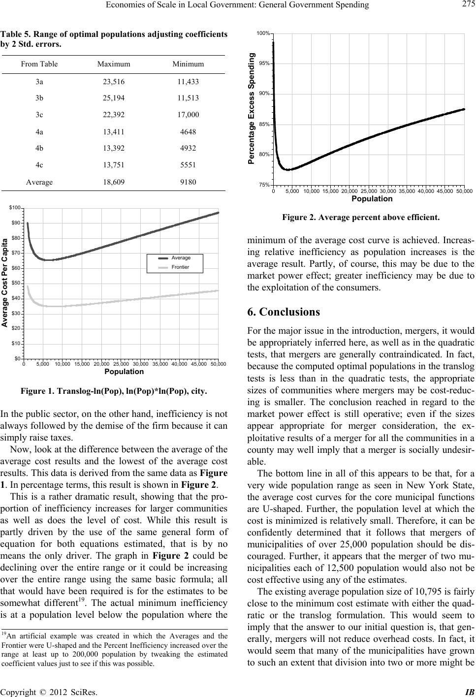

Economies of Scale in Local Government: General Government Spending 275
Table 5. Range of optimal populations adjusting coefficients
by 2 Std. err or s.
From Table Maximum Minimum
3a 23,516 11,433
3b 25,194 11,513
3c 22,392 17,000
4a 13,411 4648
4b 13,392 4932
4c 13,751 5551
Average 18,609 9180
$0
$10
$20
$30
$40
$50
$60
$70
$80
$90
$100
05,00010,000 15,000 20,000 25,000 30,000 35,000 40,000 45,000 50,000
Average Cost Per Capita
Population
Average
Frontier
Figure 1. Translog-ln(Pop), ln(Pop)*ln(Pop), city.
In the public sector, on the other hand, inefficiency is not
always followed by the demise of the firm because it can
simply raise taxes.
Now, look at the difference between the average of the
average cost results and the lowest of the average cost
results. This data is derived from the same data as Figure
1. In percentage terms, this result is shown in Figure 2.
This is a rather dramatic result, showing that the pro-
portion of inefficiency increases for larger communities
as well as does the level of cost. While this result is
partly driven by the use of the same general form of
equation for both equations estimated, that is by no
means the only driver. The graph in Figure 2 could be
declining over the entire range or it could be increasing
over the entire range using the same basic formula; all
that would have been required is for the estimates to be
somewhat different19. The actual minimum inefficiency
is at a population level below the population where the
75%
80%
85%
90%
95%
100%
05,00010,000 15,000 20,00025,000 30,000 35,000 40,000 45,00050,000
Percentage Excess Spending
Population
Figure 2. Average percent above efficient.
minimum of the average cost curve is achieved. Increas-
ing relative inefficiency as population increases is the
average result. Partly, of course, this may be due to the
market power effect; greater inefficiency may be due to
the exploitation of the consumers.
6. Conclusions
For the major issue in the introduction, mergers, it would
be appropriately inferred here, as well as in the quadratic
tests, that mergers are generally contraindicated. In fact,
because the computed optimal populations in the translog
tests is less than in the quadratic tests, the appropriate
sizes of communities where mergers may be cost-reduc-
ing is smaller. The conclusion reached in regard to the
market power effect is still operative; even if the sizes
appear appropriate for merger consideration, the ex-
ploitative results of a merger for all the communities in a
county may well imply that a merger is socially undesir-
able.
The bottom line in all of this appears to be that, for a
very wide population range as seen in New York State,
the average cost curves for the core municipal functions
are U-shaped. Further, the population level at which the
cost is minimized is relatively small. Therefore, it can be
confidently determined that it follows that mergers of
municipalities of over 25,000 population should be dis-
couraged. Further, it appears that the merger of two mu-
nicipalities each of 12,500 population would also not be
cost effective using any of the estimates.
The existing average population size of 10,795 is fairly
close to the minimum cost estimate with either the quad-
ratic or the translog formulation. This would seem to
imply that the answer to our initial question is, that gen-
erally, mergers will not reduce overhead costs. In fact, it
would seem that many of the municipalities have grown
to such an extent that division into two or more might be
19An artificial example was created in which the Averages and the
Frontier were U-shaped and the Percent Inefficiency increased over the
range at least up to 200,000 population by tweaking the estimated
coefficient values just to see if this was possible.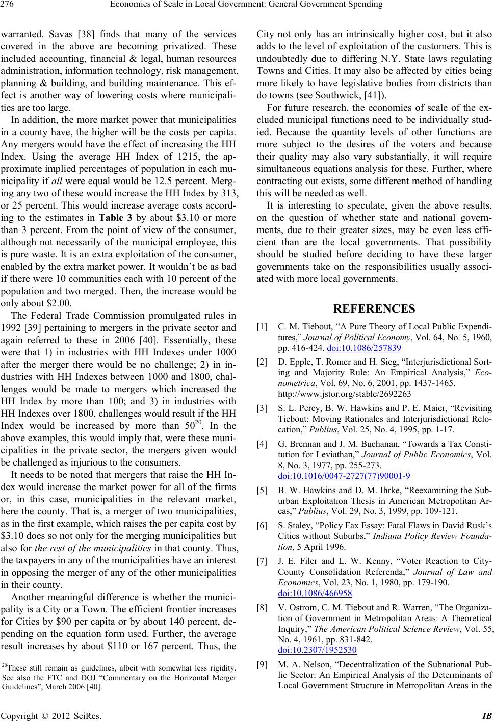

Economies of Scale in Local Government: General Government Spending
276
warranted. Savas [38] finds that many of the services
covered in the above are becoming privatized. These
included accounting, financial & legal, human resources
administration, information technology, risk management,
planning & building, and building maintenance. This ef-
fect is another way of lowering costs where municipali-
ties are too large.
In addition, the more market power that municipalities
in a county have, the higher will be the costs per capita.
Any mergers would have the effect of increasing the HH
Index. Using the average HH Index of 1215, the ap-
proximate implied percentages of population in each mu-
nicipality if all were equal would be 12.5 percent. Merg-
ing any two of these would increase the HH Index by 313,
or 25 percent. This would increase average costs accord-
ing to the estimates in Table 3 by about $3.10 or more
than 3 percent. From the point of view of the consumer,
although not necessarily of the municipal employee, this
is pure waste. It is an extra exploitation of the consumer,
enabled by the extra market power. It wouldn’t be as bad
if there were 10 communities each with 10 percent of the
population and two merged. Then, the increase would be
only about $2.00.
The Federal Trade Commission promulgated rules in
1992 [39] pertaining to mergers in the private sector and
again referred to these in 2006 [40]. Essentially, these
were that 1) in industries with HH Indexes under 1000
after the merger there would be no challenge; 2) in in-
dustries with HH Indexes between 1000 and 1800, chal-
lenges would be made to mergers which increased the
HH Index by more than 100; and 3) in industries with
HH Indexes over 1800, challenges would result if the HH
Index would be increased by more than 5020. In the
above examples, this would imply that, were these muni-
cipalities in the private sector, the mergers given would
be challenged as injurious to the consumers.
It needs to be noted that mergers that raise the HH In-
dex would increase the market power for all of the firms
or, in this case, municipalities in the relevant market,
here the county. That is, a merger of two municipalities,
as in the first example, which raises the per capita cost by
$3.10 does so not only for the merging municipalities but
also for the rest of the municipalities in that county. Thus,
the taxpayers in any of the municipalities have an interest
in opposing the merger of any of the other municipalities
in their county.
Another meaningful difference is whether the munici-
pality is a City or a Town. The efficient frontier increases
for Cities by $90 per capita or by about 140 percent, de-
pending on the equation form used. Further, the average
result increases by about $110 or 167 percent. Thus, the
City not only has an intrinsically higher cost, but it also
adds to the level of exploitation of the customers. This is
undoubtedly due to differing N.Y. State laws regulating
Towns and Cities. It may also be affected by cities being
more likely to have legislative bodies from districts than
do towns (see Southwick, [41]).
For future research, the economies of scale of the ex-
cluded municipal functions need to be individually stud-
ied. Because the quantity levels of other functions are
more subject to the desires of the voters and because
their quality may also vary substantially, it will require
simultaneous equations analysis for these. Further, where
contracting out exists, some different method of handling
this will be needed as well.
It is interesting to speculate, given the above results,
on the question of whether state and national govern-
ments, due to their greater sizes, may be even less effi-
cient than are the local governments. That possibility
should be studied before deciding to have these larger
governments take on the responsibilities usually associ-
ated with more local governments.
REFERENCES
[1] C. M. Tiebout, “A Pure Theory of Local Public Expendi-
tures,” Journal of Political Economy, Vol. 64, No. 5, 1960,
pp. 416-424. doi:10.1086/257839
[2] D. Epple, T. Romer and H. Sieg, “Interjurisdictional Sort-
ing and Majority Rule: An Empirical Analysis,” Eco-
nometrica, Vol. 69, No. 6, 2001, pp. 1437-1465.
http://www.jstor.org/stable/2692263
[3] S. L. Percy, B. W. Hawkins and P. E. Maier, “Revisiting
Tiebout: Moving Rationales and Interjurisdictional Relo-
cation,” Publius, Vol. 25, No. 4, 1995, pp. 1-17.
[4] G. Brennan and J. M. Buchanan, “Towards a Tax Consti-
tution for Leviathan,” Journal of Public Economics, Vol.
8, No. 3, 1977, pp. 255-273.
doi:10.1016/0047-2727(77)90001-9
[5] B. W. Hawkins and D. M. Ihrke, “Reexamining the Sub-
urban Exploitation Thesis in American Metropolitan Ar-
eas,” Publius, Vol. 29, No. 3, 1999, pp. 109-121.
[6] S. Staley, “Policy Fax Essay: Fatal Flaws in David Rusk’s
Cities without Suburbs,” Indiana Policy Review Founda-
tion, 5 April 1996.
[7] J. E. Filer and L. W. Kenny, “Voter Reaction to City-
County Consolidation Referenda,” Journal of Law and
Economics, Vol. 23, No. 1, 1980, pp. 179-190.
doi:10.1086/466958
[8] V. Ostrom, C. M. Tiebout and R. Warren, “The Organiza-
tion of Government in Metropolitan Areas: A Theoretical
Inquiry,” The American Political Science Review, Vol. 55,
No. 4, 1961, pp. 831-842.
doi:10.2307/1952530
[9] M. A. Nelson, “Decentralization of the Subnational Pub-
lic Sector: An Empirical Analysis of the Determinants of
Local Government Structure in Metropolitan Areas in the
20These still remain as guidelines, albeit with somewhat less rigidity.
See also the FTC and DOJ “Commentary on the Horizontal Merger
Guidelines”, March 2006 [40].

Economies of Scale in Local Government: General Government Spending 277
US,” Southern Economic Journal, Vol. 57, No. 2, 1990,
pp. 443-457.
[10] S. Falcone and Z. Y. Lan, “Intergovernmental Relations
and Productivity,” Public Administration Review, Vol. 57,
No. 4, 1997, pp. 319-322.
[11] M. Olson, “Toward a More General Theory of Govern-
mental Structure,” The American Economic Review, Vol.
76, No. 2, 1986, pp. 120-125.
[12] W. J. Lynk, “Nonprofit Hospital Mergers and the Exer-
cise of Market Power,” Journal of Law and Economics,
Vol. 38, No. 2, 1995, pp. 437-461. doi:10.1086/467338
[13] M. G. Vita and S. Sacher, “The Competitive Effects of
Not-for-Profit Hospital Mergers: A Case Study,” The Jour-
nal of Industrial Economics, Vol. 49, No. 1, 2001, pp.
63-84. doi:10.1111/1467-6451.00138
[14] P. W. Abelson, “Some Benefits of Small Local Govern-
ment Areas,” Pu blius, Vol. 11, No. 1, 1981, pp. 129-140.
[15] T. J. DiLorenzo, “George Stigler and the Myth of Effi-
cient Government,” Journal of Libertarian Studies, Vol.
16, No. 4, 2002, pp. 55-73.
[16] D. D. Kneebone, “Centralization and the Size of Govern-
ment in Canada,” Applied Economics, Vol. 24, No. 12,
1992, pp. 1293-1298.
[17] R. E. Wagner and W. E. Weber, “Competition, Monopoly,
and the Organization of Government in Metropolitan Ar-
eas,” Journal of Law and Economics, Vol. 18, No. 3,
1975, pp. 661-684.
[18] L. R. Gabler, “Population Size as a Determinant of City
Expenditures and Employment: Some Further Evidence,”
Land Economics, Vol. 47, No. 2, 1971, pp. 130-138.
doi:10.2307/3145454
[19] J. S. Zax, “Is There a Leviathan in Your Neighborhood?”
The American Economic Review, Vol. 79, No. 3, 1989, pp.
560-567.
[20] D. Joulfaian and M. L. Marlow, “Government Size and
Decentralization: Evidence from Disaggregated Data,”
Southern Economic Journal, Vol. 56, No. 4, 1990, pp.
1094-1102. doi:10.2307/1059894
[21] S. C. Deller, “Local Government Structure, Devolution,
and Privatization,” Review of Agricultural Economics,
Vol. 20, No. 1, 1998, pp. 135-154. doi:10.2307/1349539
[22] J. Rodden, “Reviving Leviathan: Fiscal Federalism and
the Growth of Government,” International Organization,
Vol. 57, No. 4, 2003, pp. 695-729.
doi:10.1017/S0020818303574021
[23] J. F. Couch, B. A. King, C. H. Gossett and J. B. Parris,
“Economies of Scale and the Provision of Public Goods
by Municipalities,” Journal of Economics and Economic
Education Research, Vol. 5, No. 3, 2004, pp. 69-79.
[24] K. G. Brempong, “Economies of Scale and Municipal Po-
lice Services: The Case of Florida,” The Review of Eco-
nomics and Statistics, Vol. 69, No. 2, 1987, pp. 352-356.
doi:10.2307/1927244
[25] A. O. Gyapong and K. G. Brempong, “Factor Substitution,
Price Elasticity of Factor Demand and Returns to Scale in
Police Production: Evidence from Michigan,” Southern
Economic Journal, Vol. 54, No. 4, 1988, 16 pages.
[26] E. Ostrom and G. P. Whitaker, “Does Local Community
Control of Police Make a Difference? Some Preliminary
Findings,” American Journal of Political Science, Vol. 17,
No. 1, 1973, pp. 48-76. doi:10.2307/2110474
[27] D. L. Sjoquist and M. B. Walker, “Economies of Scale in
Property Tax Assessment,” National Tax Journal, Vol. 52,
No. 2, 1999, pp. 207-220.
[28] J. Byrnes and B. Dollery, “Do Economies of Scale Exist
in Australian Local Government? A Review of the Em-
pirical Evidence,” Working Paper Series in Economics,
University of New England School of Economics, Armi-
dale, No. 2002-2.
[29] W. Hirsch, “Expenditure Implications of Metropolitan
Growth and Consolidation,” Review of Economics and
Statistics, Vol. 41, No. 3, 1959, pp. 232-241.
doi:10.2307/1927450
[30] B. Lockwood, “Distributive Politics and the Costs of
Centralization,” The Review of Economic Studies, Vol. 69,
No. 2, 2002, pp. 313-337.
[31] J. E. Oliver, “City Size and Civic Involvement in Metro-
politan America,” The American Political Science Review,
Vol. 94, No. 2, 2000, pp. 361-373. doi:10.2307/2586017
[32] P. Bardhan, “Decentralization of Governance and Devel-
opment,” The Journal of Economic Perspectives, Vol. 16,
No. 4, 2002, pp. 185-205.
doi:10.1257/089533002320951037
[33] E. Loehman and R. Emerson, “A Simultaneous Equation
Model of Local Government Expenditure Decisions,”
Land Economics, Vol. 61, No. 4, 1985, pp. 419-432.
[34] H. Shapiro, “Economies of Scale and Local Government
Finance,” Land Economics, Vol. 39, No. 2, 1963, pp.
175-186.
[35] L. Drake and R. Simper, “X-Efficiency and Scale Econo-
mies in Policing: A Comparative Study Using the Distri-
bution Free Approach and DEA,” Applied Economics,
Vol. 34, No. 15, 2002, 12 pages.
[36] L. Southwick Jr., “Economies of Scale and Market Power
in Policing,” Managerial and Decision Economics, Vol.
26, No. 8, 2005, pp. 461-473. doi:10.1002/mde.1230
[37] W. H. Greene, “LIMDEP, v. 8.0,” Econometric Software,
Inc., Plainview, 2002.
[38] E. S. Savas, “Privatization and Public-Private Partner-
ships,” Chatham House, New Yor, 2000, pp. 72-73.
[39] Federal Trade Commission, “1992 Horizontal Merger
Guidelines,” 1992.
http://www.ftc.gov/bc/docs/horizmer.htm
[40] Federal Trade Commission and US Department of Justice,
“Commentary on the Horizontal Merger Guidelines,”
March 2006.
http://www.ftc.gov/os/2006/03/CommentaryontheHorizo
ntalMergerGuidelinesMarch2006.pdf
[41] L. Southwick Jr., “Local Government Spending and At-
Large versus District Representation: Do Wards Result in
More Pork?” Economics and Politics, Vol. 7, No. 2, 1997,
pp. 173-203. doi:10.1111/1468-0343.00027
[42] D. C. Shoup, “Effects of Suboptimization on Urban Gov-
ernment Decision Making,” Proceedings of the Twenty-

Economies of Scale in Local Government: General Government Spending
278
Ninth Annual Meeting of the American Finance Associa-
tion, Detroit, 28-30 December 1970, pp. 547-564.
[43] R. H. Coase, “The Problem of Social Cost,” Journal of
Law and Economics, Vol. 3, No. 1, 1960, pp. 1-44.
doi:10.1086/466560