iBusiness, 2012, 4, 193-197
http://dx.doi.org/10.4236/ib.2012.43024 Published Online September 2012 (http://www.SciRP.org/journal/ib)
193
Evolutionary Gaming Analysis of Path Dependence in
Green Construction Technology Change
Xian-Feng Zhang, Chuan-Min Shuai, Pei-Song Gong, Han Sun
School of Engineering & Management, China University of Geosciences, Wuhan, China.
Received April 22nd, 2012; revised May 15th, 2012; accepted June 4th, 2012
ABSTRACT
In the context of instigating green construction technology by changing current technology practices, evolutionary game
theory is used to solve path dependence problems that yield stable equilibrium. Replicating dynamic gaming shows that
in inducing technological change some problems concerning multiple equilibrium definitely exist and that profit is the
prime motivation to use or supply new technology. The model also shows that a lock-in of a current technology can be
broken as a consequence of players’ studies.
Keywords: Green Construction Technology; Path Dependent; Evolutionary Game
1. Introduction
1.1. Green Construction Technology
Construction is a process of building in which materials
are transformed into products, such as buildings, airports
and highways, which unfortunately by its nature leads
inevitably to some level of environmental pollution, ex-
travagant energy consumption and resource depletion.
The process is outlined in Figure 1. Because construc-
tion is a necessary activity, the question arises as to how
to minimize its detrimental effects; green construction
technology (GCT) incorporates the right choices to
achieve this goal. GCT refers to a kind of sustainable
development technology enabling consumption of less
resource, less energy and to bring lighter environmental
pollution during the entire construction cycle [1]. Despite
its green credentials, GCT promotion has not however
been satisfactory. It has been rejected by many builders
simply because giving up old technologies is not to their
liking, perhaps due to the expense, inconvenience or dis-
ruption to business. In this paper, the problem confront-
ing construction builders given their technology options
is investigated using evolutionary game theory to analyze
the path dependence to stable equilibrium.
1.2. Brief View of Path Dependence Research
Research using path dependence analysis covers a rich
variety of fields. In 1975, Paul A. David of Stanford
University developed the concept of path dependence
within the context of technological change [2]. David,
along with colleague W. Brian Arthur [3-6], systematized
this idea of path dependence, establishing it as one of the
more valuable theories finding a rapid development
within modern economics. They considered that techno-
logical change was a system which was influenced by a
“positive feedback mechanism”, and that change has
several characteristics, which are itemized as follows: 1)
Multiple equilibrium—that is to say, the result of a de-
veloping system is not singular but has more than one
outcome; 2) Close-down—this refers to one technology
which, once adopted, employs income-increasing mecha-
nisms preventing it from being displaced by other tech-
nologies; 3) Non-efficient possibility—those locked-in
technologies having a strangle-hold within the market are
no longer the best choices; and 4) Path dependence—the
path of an evolutionary system is dependent on the sys-
tem’s original state and trajectory. Leibowitz and Mar-
golis (1990,1994) [7,8] thought that there were two
methods which can break this path dependence: either by
predicting the results from the different choices present
or by provided more communication on options before
choices are made. Unless the subject of economics is
unwilling to change, path dependence is inevitable.
2. The Asymmetric Replication Dynamic
Game Model of Technological Change on
GCT
Evolutionary gaming is based on several hypotheses
summarized as follows: 1) Players who adopted higher
revenue strategies will repeat their strategy more readily,
and therefore in the long run, the fraction of players who
adopt lower revenue strategies will decrease; 2) Players

Evolutionary Gaming Analysis of Path Dependence in Green Construction Technology Change
194
Figure 1. The impact of construction on environment, resources and energy.
may usually imitate other players’ behaviors, and posi-
tive correlations may ensue between their revenues and
their imitative tendencies; and 3) When one player chan-
ges strategy, they always treat the present situation as a
known condition, and then change to a kind of corre-
sponding best strategy.
Given the above hypotheses, an asymmetric replica-
tion dynamic game model is considered to analyze the
process of instigating change to GCT. Assuming there
are two groups of players: one group comprising the
GCT (GCTs, for instance manufacturers, which we here
denote by F (we do not know a priori whether the tech-
nology used is GCT or not); the other group comprising
the technology users, for instance consumers which we
here denote by C. We assume two techniques can be
chosen in the market. The strategies of GCTs are SF =
{S1, S2}, where S1, and S2 mean those GCTs choosing
technique 1 and technique 2, respectively. The strategy
space of the technology users is SC = {S1, S2}, where the
Si denote the same as above. For this situation we can
form a matrix game by establishing pay-offs between
random pairings of GCTs and users (see Figure 2).
Here we let A, C denote profits to be gained when sup-
pliers choose technique 1 while E, G denote the same
when technique 2 is chosen. The benefits to users are
denoted as B, D, F and H as above. In addition, we as-
sume technique 2 can gain more profit than technique 1,
that is to say, A < B, C < D.
At the start of the Game, the fraction of suppliers
adopting technique 1 is p while the difference 1 − p
represents those adopting technique 2. Similarly, the
fraction of technology users adopting technique 1 is q,
while 1 − q corresponds to those adopting technique 2.
Let uf1 be the expected revenue when the GCTS choose
technique 1 and uf2 the expected revenue of those choos-
ing technique 2. The average revenue is denoted by
f
u.
User
S
1 S 2
S1 A, B C, D
GCTs
S2 E, F G, H
Figure 2. Pay-off matrix of user-supplier.
We then have the following set of consistency relations:

*
*
11 f
uqA qC
G

(1)

*
*
21 f
uqE q (2)


*
*
12
1
11
ff f
upu pu
A
EpqC Gpq



(3)
Similarly, revenues for the technology users satisfy a
set of like relations:

*
*
11 c
upB pD


*
21
c
upF pH



 
*
*
12
1
11
cc c
uqu qu
BFpq DHpq



From evolutionary gaming theory, we can develop the
replicated dynamic equation for both groups associated
with the two positions. This leads to the GCTS’ repli-
cated dynamic equation:

 
12
d
d
11
ff
ppu u
t
ppAEqGC qFy

 


(4)
If


qBAB

, then ddpt will always be 0, that
is to say, all the p are stable. If

qBAB, then

Evolutionary Gaming Analysis of Path Dependence in Green Construction Technology Change 195
*0q
1p
and are two stable states of p, for which
is an evolutionary stable strategy. If
*1p


qBAB,
then and are still the two stable states
of p, but for which now becomes the evolution-
ary stable strategy.
*0p*1
*0p
p
Likewise, the replicated dynamic equation of the tech-
nology users group is:

cc
u


d1
d
qqCDp D
t 

1
qu

q

(5)
If pDCD , then dd 0pt; that is to say, all
values of p are stable. If

ppDCD , then *0q

and are two stable states of q, with
*
q11q

being
the evolutionary stable strategy. If


ppD CD,
then and are again two stable states of p,
with the evolutionary stable strategy. The pro-
portional change and replicator dynamics are shown in
Figure 3.
*
q
q0
*0
*
q1
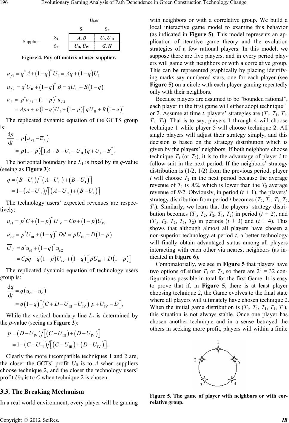
From Figure 3, we find that this game will converge
to points (0, 0) and (1, 1). These two points correspond to
two equilibrium points: respectively, one is *0p

and
, the other and . In Figure 3, the
graph is divided into four regions by lines L1 and L2. The
analysis is as follows: 1) When the initial state falls
within the left inferior region, that is to say, the fraction
of GCTs less than
*0q*1

p*1q

DC D and the fraction of tech-
nology users less than


BAB that have changed
choice to technique 1. In this situation the Game will
eventually converge to the evolutionary stable strategy
and , and technique 1 will eventually not
be totally adopted; 2) When the initial state falls within
the right superior region, the fraction of GCTs is greater
than
*0p*0q

DC D and the fraction of technology users is
greater than

BAB, and both groups begin to
choose technique 1. As a consequence the Game will
eventually converge to the evolutionary stable strategy
and q, and technique 1 will eventually be
adopted in total; 3) When the initial state falls within
either the left superior region or the right inferior region,
the Game will converge to point (0, 0) or (1, 1). The final
*1p*1
Figure 3. The connection between proportional change and
replicator dynamics of the two types of groups.
equilibrium state is dependent on the speed that the
groups learn and adjust. When the state falls within the
left superior region and the evolution dynamics passes
through line L1 arriving at the right superior region first,
the final equilibrium will be and
*0p*0q

; in
contradistinction, if the evolution dynamics passes
through line L1 and arrives at the left inferior region first,
the final equilibrium will be and
*1p*1q

; in re-
gard to the right inferior and left superior regions, the
evolution dynamics are just mirror opposites.
By the above model analysis, we can see clearly that
different initial states will lead to different equilibrium.
At the initial stage, the probability bias in adopting one
of several techniques compels the process of technologi-
cal change or locks the process of GCT changes towards
an equilibrium point of game. Evolution has several po-
tential outcomes based on multiple equilibriums.
3. Game Analyses on Breaking Technology
Lock-In
Although the asymmetric replication dynamic game
model above explains the reason of multiple equilibrium
and tells us why subdominant option technology can be
used during technological changes, however, the model
needs to be modified to pay more attention to several real
world issues which we now present.
3.1. The Situation of New Players Joining
When a new player adopting technique 2 is added to the
original technology users group, the total population will
increase. The addition may make the proportion adopting
technique 2 exceed


BAB, which in turn makes the
group that had adopted technique 1 opt for technique 2.
Likewise, when a new exotic player opting for technique
2 is added to the original technology supplier group, and
the fraction adopting technique 2 now exceeds


DC D

,
the technology suppliers group that had adopted tech-
nique 1 will also convert to technique 2 with similar
consequences.
3.2. The Result on Technology Compatibility
If some compatibility between techniques 1 and 2 exists,
the revenues for both GCTs and technology users will no
longer be zero when they both choose technique 2. We
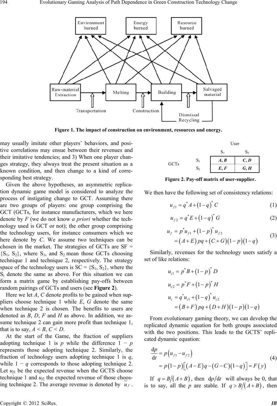
need to modify the pay-off matrix in Figure 1 to that
shown in Figure 4. Here both UI and UII are less than A,
and both UIII and UIV are less than C. We had supposed
A < B and C < D previously, so we can conclude that UI
< A < B, UII < A < B, UIII < C < D and UIV < C < D.
Here, the expected revenues when the GCTs choose
either technique 1 or technique 2 are uf1 and uf2 respec-
tively. The average revenue is denoted as
f
u. The con-
sistency relations become:

Evolutionary Gaming Analysis of Path Dependence in Green Construction Technology Change
196
User
S
1 S 2
S1 A, B UI, UIII
Supplier
S2 UII, UIV G, H
Figure 4. Pay-off matrix of user-supplier.
 
*
*
1I
11
f
uqA qUAqqU I
  
*
*
2II II
11
f
uqU qBqUBq

 
*
*
12
III
1
11 1
ff f
upu pu
A
pqpq UpqUBq

 
 
The replicated dynamic equation of the GCTS group
is:

 
1
IIII
d
d
1
ff
ppu u
t
.
p
pABUUqUB

 
 
The horizontal boundary line L1 is fixed by its q-value
(seeing as Figure 3):
 

IIII
IIII I
1
qBU AU BU
AUAU BU
  

   

The technology users’ expected revenues are respec-
tively:
 
*
*
1IV
11
c
upCpUCp pUIV

1
 
*
*
2 IIIIII
1
c
upU qDdpUDp 

 
*
*
12
IV III
1
11 1
fcc
Uqu qu
Cpqq pUqpUDp

  
 
The replicated dynamic equation of technology users
group is:

 
1
III IVIV
d
d
1
cc
qqu u
t
qqCDUUpUD


 
,


While the vertical boundary line L2 is determined by
the p-value (seeing as Figure 3):
 


 
IVIII IV
III III IV
1.
pDUCU DU
CUCU DU

 


 



Clearly the more incompatible techniques 1 and 2 are,
the closer the GCTs’ profit UII is to A when suppliers
choose technique 2, and the closer the technology users’
profit UIII is to C when technique 2 is chosen.
3.3. The Breaking Mechanism
In a real world environment, every player will be gaming
with neighbors or with a correlative group. We build a
local interactive game model to examine this behavior
(as indicated in Figure 5). This model represents an ap-
plication of iterative game theory and the evolution
strategies of a few rational players. In this model, we
suppose there are five players, and in every period play-
ers will game with neighbors or with a correlative group.
This can be represented graphically by placing identify-
ing marks say numbered stars, one for each player (see
Figure 5) on a circle with each player gaming repeatedly
only with their neighbors.
Because players are assumed to be “bounded rational”,
each player in the first game will either adopt technique 1
or 2. Assume at time t, players’ strategies are (T1, T1, T1,
T1, T2). That is to say, players 1 through 4 will choose
technique 1 while player 5 will choose technique 2. All
single players will adjust their strategy simply, and this
decision is based on the strategy distribution which is
given by the players’ neighbors. If both neighbors choose
technique T1 (or T2), it is to the advantage of player i to
follow suit in the next period. If the neighbors’ strategy
distribution is (1/2, 1/2) from the previous period, player
i will choose T2 in the next period because the average
revenue of T1 is A/2, which is lower than the T2 average
revenue of B/2. Obviously, in period (t + 1), the players’
strategy distribution from period t becomes (T2, T1, T1, T2,
T1). Similarly, we learn that the players’ strategy distri-
bution becomes (T1, T2, T2, T1, T2) in period (t + 2), and
(T1, T2, T2, T1, T2) in periods (t + 3) and (t + 4). This
shows that although almost all players have chosen a
non-superior technology at period t, a better technology
will finally obtain advantaged status among all players
interacting with each other via nearest neighbors (as in-
dicated in Figure 6).
Combinatorially, we see in Figure 5 that players have
two options of either T1 or T2, so there are 25 = 32 con-
figurations possible in total for the first Game. It is easy
to prove that if, in Figure 5, there is at least player
choosing technique 2, the Game evolves to the final state
where all players will ultimately have chosen technique 2.
When the initial game distribution is (T1, T1, T1, T1, T1),
this situation is not always stable. Once one player has
chosen another technique and in a sense betrayed the
others in seeking more profit, players will within a finite
Figure 5. The game of player with neighbors or with cor-
relative group.

Evolutionary Gaming Analysis of Path Dependence in Green Construction Technology Change
197
Figure 6. GCT strategic distributions.
REFERENCES
period draw closer to the state (T2, T2, T2, T2, T2) em-
ploying the better technology. According to this theo-
retical analysis, all non-superior technologies will ulti-
mately be replaced by the more efficient technologies.
[1] X. F. Zhang, “A New Challenge in Construction Man-
agement—The Sustainable Development,” Resource, En-
vironment and Projection, Vol. 9, 2004, pp. 88-91.
[2] H. P. Young, “The Evolution of Conventions,” Econo-
metrica, Vol. 61, No. 1, 1993, pp. 57-84.
4. Conclusions
[3] W. B. Arthur, “Competing Technologies, Increasing Re-
turns and Lock-In by Historical Events,” The Economic
Journal, Vol. 99, 1989, pp. 116-131.
1) The model presented shows that, in instigating a
process of technological change, several problems in
regarding to multiple equilibriums definitely exist. In
competition, the final result of the dynamic evolution is
that one of several techniques either occupied the market
totally or has no market share. Which of the techniques
will dominate is however hard to predict as the results of
the Game are affected directly by its initial states. This
model has though explained the path dependence in in-
stigating technological change.
[4] W. B. Arthur, “Increasing Returns and Path Dependence
in the Economy,” University of Michigan Press, Ann Ar-
bor, 1994.
[5] P. A. David, “Clio and the Economics of Qwerty,” Ameri-
can Economic Review, Vol. 75, 1985, pp. 332-337.
[6] P. A. David, “Some New Standards for the Economics of
Standardisation in the Information Age,” In: P. Dasgupta
and P. Stoneman, Eds., Economic Policy and Technologi-
cal Performance, Cambridge University Press, Cambrid-
ge, 1987. doi:10.1017/CBO9780511559938.010
2) On questions of whether lock-in of subdominant op-
tional technology can be broken, three principle situa-
tions have been discussed: the addition of new players,
technology compatibility and several learning players.
All of these situations indicated that the close-down state
of subdominant optional technology is unstable under
certain environments, and that more efficient techniques
will eventually replace subdominant option technology.
[7] S. Leibowitz and S. Margolis, “The Fable of the Keys,”
Journal of Law & Economics, Vol. 33, No. 1, 1990, pp.
1-25. doi:10.1086/467198
[8] S. Leibowitz and S. Margolis, “Network Externality: An
Uncommon Tragedy,” Journal of Economic Perspectives,
Vol. 8, No. 2, 1994, pp. 133-150. doi:10.1257/jep.8.2.133