Journal of Modern Physics
Vol.3 No.9A(2012), Article ID:23118,9 pages DOI:10.4236/jmp.2012.329166
Time Evolution of Horizons
Department of Physics and Astronomy, University of Lethbridge, Lethbridge, Canada
Email: arundhati.dasgupta@uleth.ca
Received June 24, 2012; revised July 25, 2012; accepted August 2, 2012
Keywords: Black Hole Physics; Quantum Gravity; Hawking Radiation; Loop Quantum Gravity; Coherent States
ABSTRACT
Finding the origin of Hawking radiation has been a puzzle to researchers. Using a loop quantum gravity description of a black hole slice, a density matrix is defined using coherent states for space-times with apparent horizons. Evolving the density matrix using a semi-classical Hamiltonian in the frame of an observer outside the horizon gives the origin of Hawking radiation.
1. Introduction
A new theory is expected to take over at Planck distances as “quantum effects” of gravity start dominating. One of the promising approaches to the theory of quantum gravity is the theory of Loop Quantum Gravity (LQG), which is by formulation non-perturbative and background independent [1-3]. LQG has a well defined kinematical Hilbert space, and though the Hamiltonian constraint remains unsolved, the theory allows for a semiclassical sector of the theory. This includes “coherent states” [4,5] which are peaked at classical phase space elements. Using these as a starting point, I defined in a series of papers [6-8] coherent states for the Schwarzschild spacetime, and derived an origin of entropy using quantum mechanical definition of entropy from density matrices. The exact entropy is a function of the graph used to obtain the LQG phase space variables [9]. The zeroeth order term is proportional to the area of the horizon signifying a universality of the Bekenstein-Hawking entropy. The proportionality constant and the correction terms bring out the details of the graph [8].
In this paper we take this new way of finding the origin of entropy a step further by evolving the spatial slice in time [10], and observing the evolution of the density matrix in the process. This state as of now does not satisfy the Hamiltonian constraint, but one is allowed to take an arbitrary initial state, or a wavepacket with appropriate properties, representing a macroscopic configuration. The evolution discussed in this paper is semiclassical, i.e. no attempt is made to use the full Hamiltonian.
The quasilocal energy (QLE) of an outside observer, defined in [11] is used as the Hamiltonian to evolve the system. As the time clicks in the observers clock, the Hamiltonian evolves the coherent state such that the area of the horizon remains the same as predicted by classical physics. However, classically forbidden regions become accessible quantum mechanically, and vertices of the graph hidden behind the horizon in one slice emerge outside the horizon in the next slice. This gives a net change in area, and the mass deficit is emitted from the black hole. This evolution is not unitary, and the quasi-local energy which is used to evolve the slice is not mapped to a Hermitian operator. When matter is coupled to the gravitational system, a net flux emerges causing a decay of the horizon.
In Section 2 we introduce the formalism by describing the coherent state, the black hole time slice, the apparent horizon equation, and the density matrix. Section 3 describes the time evolution of the system and gives a derivation of the change in entropy. In Section 4 we give a description of a matter current emergent from behind the horizon. Finally in the concluding section we include a discussion about the implications of the nonHermitian evolution.
2. The Coherent State in LQG
For gravity, finding the canonical variables which describe the physical phase space is an odd task as there is no unique time. Nevertheless a fiducial time coordinate can be chosen, which breaks the manifest diffeomorphism invariance, restored in the Hilbert space of states by imposing constraints.
The constant time slices are described by the intrinsic metric  and the extrinsic curvature
  (a,b = 1,2,3). The theory can be formulated in terms of the square root of the metric, the triads
  defined thus:
 (1)
(1)
where  represents the internal index for the rotation group SO(3) of the tangent space and
 . The internal group is taken to be SU(2), as this is locally isomorphic to SO(3). The theory is then defined in terms of the “spin connection”
  and the triads. However, a redefinition of the variables in terms of tangent space densitised triads
  and a corresponding gauge connection
  where I represents the SU(2) index simplifies the quantisation considerably.
 (2)
(2)
( are the usual triads,
  is the extrinsic curvature,
  the associated spin connection,
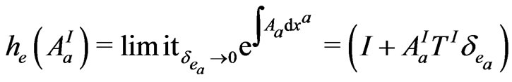
  the one parameter ambiguity which remains named as the Immirzi parameter). The quantisation of the Poisson algebra of these variables is done by smearing the connection along one dimensional edges
  of length
  of a graph
  to get holonomies
 . The triads are smeared in a set of 2-surface decomposition of the three dimensional spatial slice to get the corresponding momentum
 . The algebra is then represented in a kinematic “Hilbert space”, in which the physical constraints have been “formally” realised [12]. Once the phase space variables have been identified, one can write a coherent state for these [4] i.e. minimum uncertainty states peaked at classical values of
 . In analogy with the harmonic oscillator coherent states, where the coherent state is a function of the complexified phase space element
 , the SU(2) coherent states are peaked at the complexified phase space element
 . These
  are thus elements in the complexification of SU(2) as
  (
( being the generator matrices of SU(2)) is a Hermitian matrix and
  is the unitary SU(2) matrix. Whether these are physical coherent states, or have appropriate behavior under the action of the constraints has to be examined carefully [13]. The coherent state in the momentum representation for one edge is defined to be
 (3)
(3)
In the above  is a complexified classical phase space element
 , (the
  and the
  represent classical momenta and holonomy obtained by embedding the edge in the classical metric). The
are the usual basis spin network states given by which is the jth representation of the SU(2) element
 . Similarly,
  dimensional representations of the
  matrix
  are denoted as
 . The j is the quantum number of the SU(2) Casimir operator in that representation, and
  represent azimuthal quantum numbers which run from
 . The coherent state is precisely peaked with maximum probability at the
  for the variable
  as well as the classical momentum
  for the variable
 . The fluctuations about the classical value are controlled by the parameter t (the semiclassicality parameter). This parameter is given by
  where
where  is Planck’s constant and a a dimensional constant which characterises the system. The coherent state for an entire slice can be obtained by taking the tensor product of the coherent state for each edge which form a graph
 ,
,
 (4)
(4)
In [7] the  was evaluated for the Schwarzschild black hole by embedding a graph on a spatial slice with zero intrinsic curvature. The particular graph which was used had the edges along the coordinate lines of a sphere. This simplistic graph, was very useful in obtaining the description of the space-time in terms of discretised holonomy and momenta. A particularly interesting consequence of this was that the phase space variables were finite and well defined even at the singularity.
Given that the area of a surface in gravity is measured as the integral of the square root of the metric over the surface, the area operator can be written simply as  . The expectation value of the area operator in the coherent state emerges as [9]
 (5)
(5)
Thus we are considering a semiclassical state, which is a state such that expectation values of operators are closest to their classical values. The information of the classical phase space variables are encoded in the complexified SU(2) elements labeled as . The fluctuations over the classical values are controlled by the semiclassical parameter t.
The density matrix which describes the entire black hole slice is obtained as
 (6)
(6)
where  is the coherent state wavefunction for the entire slice, a tensor product of coherent state for each edge.
2.1. Apparent Horizons
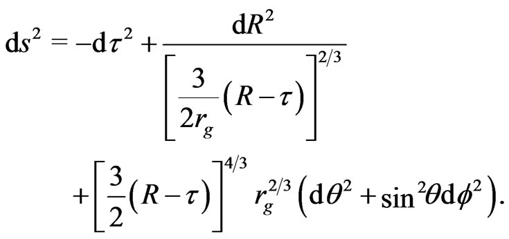
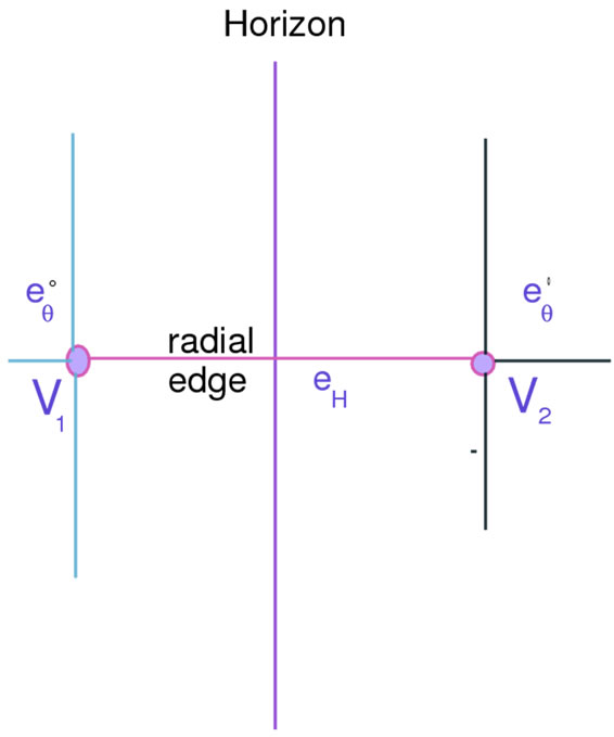
We concentrate on the coherent state near the apparent horizon contained in the spatial slice. We find that motivated from the apparent horizon equation the graph across the horizon can be taken to be populated by radial edges, linking vertices outside and inside the horizon. One then traces over the coherent state within the horizon. Initially we take a particular time slicing of the black hole, which has the spatial slices with zero intrinsic curvature [7]. One such metric which has the time slices as flat is the Lemaitre metric
 (7)
(7)
The , (in units of c = 1) and in the
  constant slices one can define the induced metric in terms of a “r” coordinate defined as
( ) on the slice. One gets the metric of the three slice to be
 (8)
(8)
The entire curvature of the space-time metric is contained in the extrinsic curvature or 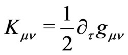 tensor of the
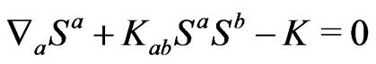
  constant slices. Now if there exists an apparent horizon somewhere in the above spatial slice, then that is located as a solution to the equation
 (9)
(9)
where , (
, ( denote the spatial indices) is the normal to the horizon,
  the extrinsic curvature in the induced coordinates of the slice, and
  the trace of the extrinsic curvature. If the horizon is chosen to be the 2-sphere, then in the coordinates of (8),
  , the apparent horizon equation as a function of the metric reduces to:
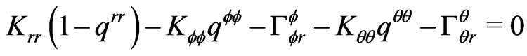 (10)
(10)
Note that the first term of the equation disappears trivially as 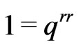 for any point in the spatial slice. Even at the operator level the
  can be set to the identity operator in the first approximation, as
 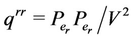 (
( being the volume operator) upto normalisations, and in the spherically symmetric metric
 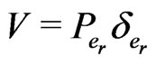 (upto discretisation constants). Thus the operators in the numerator and denominator cancel and the normalisation conspire, leaving
 . To understand the rest of the equation in terms of the holonomy and momentum variables of LQG, which are classically measured in the same metric as (8), we use the following regularisation
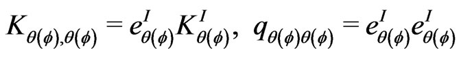 (11)
(11)
 (12)
(12)
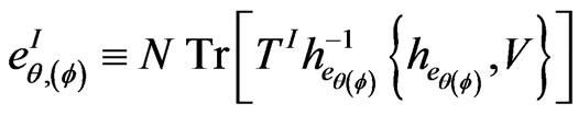
(N is a constant, a function of the edge lengths and the area bits of the discretisation) and V is the volume operator.
 (13)
(13)
Here  has been used as a parameter to identify the
  operator, and this is mainly a trick. In the continuum limit
 (14)
(14)
As the gauge connection is a function of the Immirzi parameter due to (2), the expectation value of this operator in a coherent state will be a function of the Immirzi parameter. By taking the derivative wrt to the Immirzi parameter we are giving the same status to the parameter as is given to “dimension” in a dimensional regularisation of Feynman diagrams. We let the parameter vary by an infinitesimal amount from its value in the particular quantisation sector, take the derivative, and put its original value in the final answer for the  operator. The Formula (13) is facilitated by the fact that the dependence of
  on the
  is linear. One way to check whether this gives the proper answer is to take a solved quantum mechanical system and use a similar method there. The most useful example is the Harmonic Oscillator Hamiltonian, which can be written as
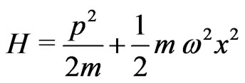 (15)
(15)
The ground state is a coherent state, so we take that as an example. We define the operator
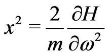 (16)
(16)
Thus
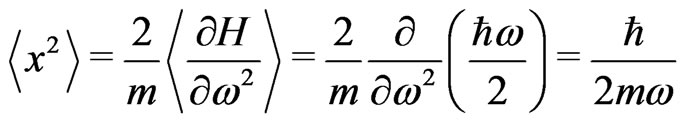 (17)
(17)
The regularisation (13) is thus an allowed approximation.
The terms involving the Christoffel connections like  include derivatives in the regularised version, the derivatives appear as difference of triads across two vertices. Thus
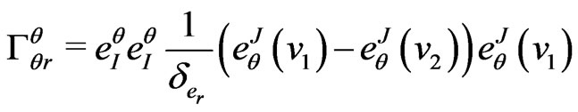 (18)
(18)
As a result of this if we impose restrictions on the Christoffel connections and one of the vertices  is within the horizon, whereas
  is outside the horizon, there will be correlations across the horizon.
If one evaluates the expectation value of the apparent horizon equation using the regularised variables in the coherent states, then one would obtain
 (19)
(19)
( is a constant).
2.2. Density Matrix
The density matrix is obtained as
 (20)
(20)
where  is the coherent state wavefunction for the entire slice, a tensor product of coherent state for each edge.
But given this, we concentrate in a “local” region to see the behavior of the horizon
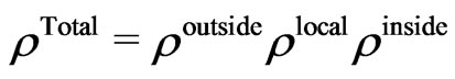 (21)
(21)
where  covers a band of vertices surrounding the horizon one set on a sphere at radius
  and one set on a sphere at radius
  within the horizon, as described in [9], and in the figure enclosed. This local density matrix and the correlations due to the apparent horizon equation (19) was used to derive entropy [6]. This entropy counts the number of ways to induce the horizon area using the spin networks, though the constraints have not been appropriately imposed as was obtained using a Chern-Simons theory in [14]. However, the entropy calculation using the coherent states provides a tracing mechanism, and a method to obtain correlations across the horizon which are gravitational in origin. We will henceforth deal with
 , but we will drop the local label for brevity.
3. Time Evolution
In physical systems, the Hamiltonian generates time evolution, but in General Theory of Relativity, the Hamiltonian is a constraint and generates diffeomorphisms in the time direction. So the question is, what is physical time, and if that exists, what would be the operator evolving the system in that direction? In case of space-times with time like Killing vectors, notion of time can be identified with the Killing direction, and a notion of “quasilocal energy” (QLE) defined using the same. The QLE then generates translations in the Killing time. In case of the Schwarzschild space-time, the QLE has been defined in [11]. We build the Hamiltonian which evolves the horizon from one time slice to the next by appropriately regularising the QLE. Note the “Killing time” and QLE are classical concepts, and thus regularising QLE gives us a “semiclassical” Hamiltonian.
3.1. Change in Entropy
Before we get into the analysis of what QLE evolution means, we take a simple system made up of two subsystems, and examine the consequences of a Hamiltonian evolution. Let the density matrix be defined for a system whose states are given in the tensor product Hilbert space  and given by
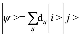 (22)
(22)
where  is the basis in
  and
and  is the basis in
  and
and  are the non-factorisable coefficients of the wavefunction in this basis. Let us label the wavefunction at time
  to be given by the coefficients
 . The density matrix is
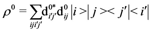 (23)
(23)
The reduced density matrix if one traces over  is:
is:
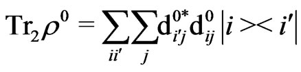 (24)
(24)
We now evolve the system using a Hamiltonian which has the matrix elements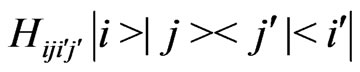 , we assume that the Hamiltonian does not factorise, that is there exists interaction terms between the two Hilbert spaces. The evolution equation is:
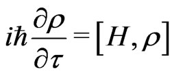 (25)
(25)
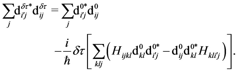
which in this particular basis gives the density matrix elements at a infinitesimally nearby slice to be
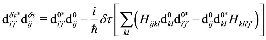 (26)
(26)
Thus we evolve the “unreduced” density matrix and then trace over the  in the evolved slice. The reduced density matrix in the evolved slice is:
 (27)
(27)
This gives:
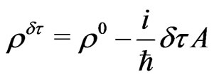 (28)
(28)
where A represents the commutator. Clearly the entropy in the evolved slice evaluated as
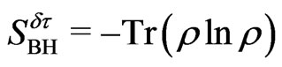
can be found as
 (29)
(29)
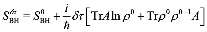
Given the definition of , one gets
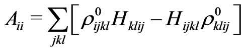 (30)
(30)
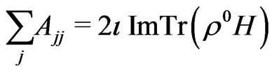
In case both the Hamiltonian and the density operator are Hermitian, one obtains
 (31)
(31)
This is clearly calculable, and gives the change in entropy . The
. The  term yields corrections, and we ignore it in the first approximation.
3.2. The Hamiltonian
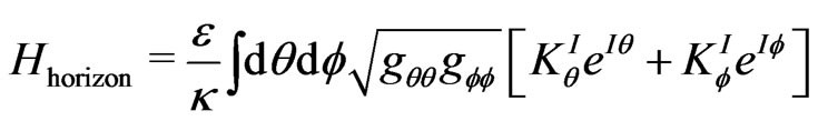
To trace the origin of Horizon fluctuations, we must take an observer who is stationed outside the horizon, or in other words is not a freely falling observer. The quasilocal energy is defined using a “surface” integral of the extrinsic curvature with which the surface is embedded in three space. In our case, we take the bounding surface to be the horizon and the quasilocal energy is given by the surface term [11,15].
 (32)
(32)
where  is the extrinsic curvature with which the 2- surface, which in this case is the horizon
  is embedded in the spatial 3-slices, and
  is the determinant of the two metric
  defined on the 2-surface. This “quasilocal energy” is measured with reference to a background metric. Thus
 . We concentrate on the physics observed in an observer stationed at a r = constant sphere.
The metric in static  observer’s frame is
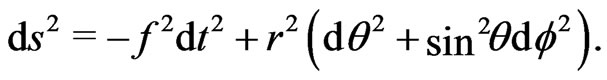 (33)
(33)
The  where
where  is the Schwarzschild radius. If we take
  to be the space-like vector, normal to the 2-surface, then the extrinsic curvature is given by:
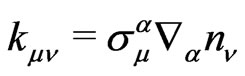 (34)
(34)
and the trace is obviously
 (35)
(35)
In the special slicing of the of the stationary observer the normal to the horizon 2-surface is given by  . However, we built the coherent state on the Lemaitre slice. The Lemaitre and the Schwarzschild observer’s coordinates are related by the following coordinate transformations,
 (36)
(36)
The r = const cylinder of the Schwarzschild coordinate corresponds to  of the Lemaitre coordinates, and for these
 . Thus unit translation in the t coordinate coincides with unit translation in the
  coordinate. Further, the intersection of the r = constant cylinder with a t = constant surface coincides with the intersection of r = constant and the
  = constant surface. Thus in the initial slice, the QLE Hamiltonian can be written as
 (37)
(37)
The reference frames’ quasilocal energy is a number, it just defines the zero point Hamiltonian. Thus, we replace the classical expressions by operators evaluated at the  = constant slice. In the first approximation we simply take the
  as classical
 as this arises due to the coordinate transformation and the norm of the vector
  in the previous frame. In the rewriting of (37) in regularised LQG variables the Hamiltonian appears rather complicated.
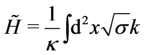
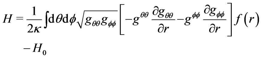
One can rewrite these in a much simpler form, using the apparent horizon equation. Since the Hamiltonian is an integral over the horizon, the variables will satisfy the apparent horizon Equation (10) upto quantum fluctuations. Thus the Hamiltonian operator is then re-written as
 (38)
(38)
where we have used the classical apparent horizon equation (10) (with ).
).
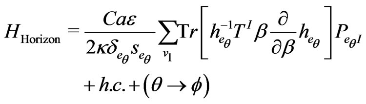 (39)
(39)
where  consists of some dimensionless constants
  is the 2-dimensional area bit over which
  is smeared,
  is a dimensionfull constant which appears to get the
  dimension less.
  is the length for the angular edge
  over which the gauge connection is integrated to obtain the holonomy. The sum over
  is the set of vertices immediately outside the horizon. The (39) can then be lifted to an operator.
This regularised expression for QLE is for the horizon 2-surface only and would not apply for any other spherical surface in the Schwarzschild space-time.
3.3. U(1) Case
Let us take the U(1) case to make the calculations easier and observe the action of the QLE Hamiltonian on the evolution of the coherent state. The spin network states are replaced by ,
,  , n is an integer and the coherent states are:
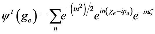 (40)
(40)
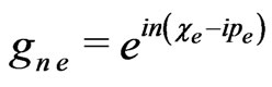 is the complexified phase space element in the “n-th” representation.
The QLE operator also takes the simplified form
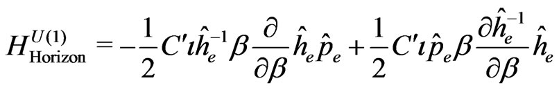 (41)
(41)
The prefactors have been clubbed into .
.
In the calculation of the matrix elements, we drop the label of the edges  for the Hamiltonian.
 (42)
(42)
This calculation can be done by putting an assumption that the . In this
  are completely independent of
 . It is an allowed assumption, and identifies the
  dependence of the operator matrix elements, which are otherwise “hidden”. The calculation however introduces an arbitrariness in the formula, which can be fixed by requiring that the expectation value of the Hamiltonian agrees with the classical QLE [10]. However, in this paper we use the “annihilation” operators defined in [16].
This is done by observing that the U(1) coherent states are eigenstates of an annihilation operator defined thus:
 (43)
(43)
The holonomy operator can thus be written as
 (44)
(44)
And the derivative wrt Immirzi parameter of the holonomy which appears in the definition of the Hamiltonian replaced by
 (45)
(45)
The dependence of the operator  on the Immirzi parameter is known (2), and thus we could evaluate the derivative
The term
 (46)
(46)
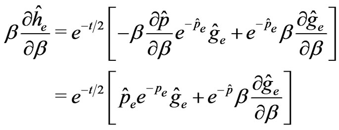
is then computable. Let us take the first term of (41) and find (46). As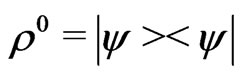 , (46) gives simply (we drop the “e” label for brevity)
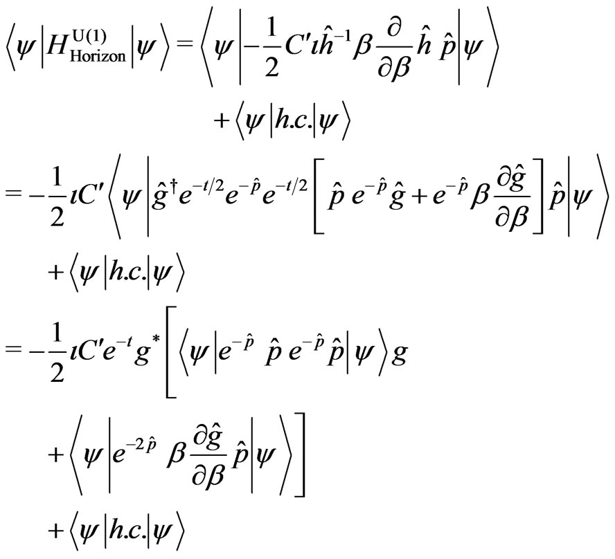
We then concentrate on the 2nd term of the above
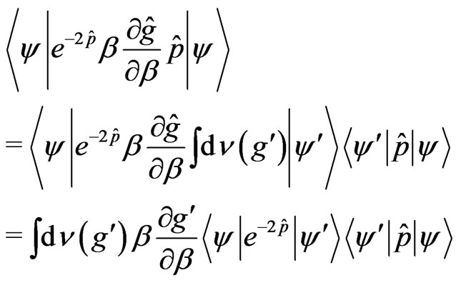 (47)
(47)
where we have used the fact that coherent states resolve unity. It can be shown that the expectation value of the operators in the  collapses the integral to
  point [16]. Thus one obtains from the above
 (48)
(48)
which is real, and thus
 (49)
(49)
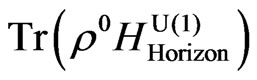
this is actually the classical QLE as it should be from .
.
This is obvious, as the way the Hamiltonian is defined, this is simply a function of the Hilbert space outside the horizon, and the matrix elements of this will not yield anything new. We approximated the horizon sphere by summing over  vertices immediately outside the horizon. We could do the same by summing over
  vertices immediately within the horizon. For the Lemaitre slice, the metric is smooth at the horizon, and one can take the “quantum operators” evaluated at the vertex
 . In this case however, as the region is within the classical horizon, the norm of the Killing vector is negative, and
  has components which are imaginary. The
 .
.
Thus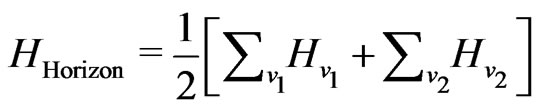 . In the evaluation of the QLE, the energy would emerge correct in the
  limit as
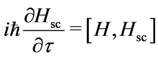
  The regularised Hamiltonian is not Hermitian, and the evolution equation is
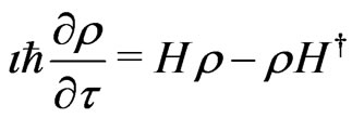 (50)
(50)
And thus the operator which appears in the change of entropy equation is
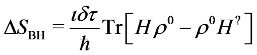 (51)
(51)
 (52)
(52)
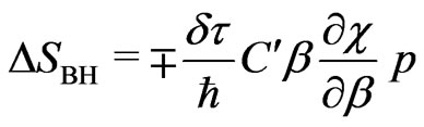
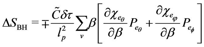
The “rate of change” of entropy is thus
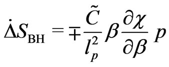 (53)
(53)
we extracted the  from
from  to get
  and rewrote the rest of the constants as
 .
.
Thus there is a net change in entropy, but, to see if this is Hawking radiation, we have to couple matter to the system.
3.4. SU(2) Case
The SU(2) case is easily reduced to the U(1) case in the actual calculation due to the gauge fixing. This is achieved by making the following observations: To retain the metric as in the same form as the classical metric, we impose the conditions at the operator level
 (54)
(54)
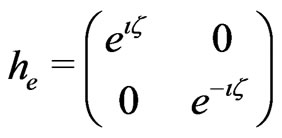
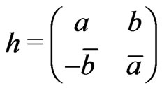
such that the corresponding metric has only the diagonal terms as non-zero. With these additional “constraints” on the operators, we can put the  such that each has only one component surviving, let’s say
 . This also makes the holonomy restricted to the U(1) case, as the gauge connection
  gets restricted to the
  and other directions can be put to zero. Thus we can take the holonomy to be diagonal. If the holonomy matrix is off-diagonal the U(1) projection still works out to be the same
 (55)
(55)
The operator is then obtained as
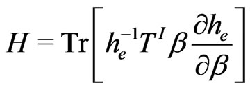
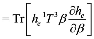
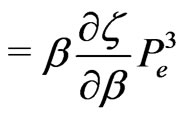 (56)
(56)
This is same as the U(1) Hamiltonian (upto normalisations). The spin network states also project on to U(1) subgroup, thus giving us the same techniques to use in the calculation of the U(1) states as for this one. To observe this, the non-zero elements for the holonomy matrix
 (57)
(57)
in the j-th representation is given by:
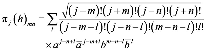 (58)
(58)
Clearly in the particular case we are considering, the , and m, n = –j and j. Thus the two non-zero elements are
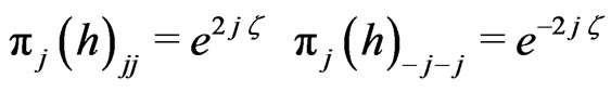 (59)
(59)
The sum over j in the  with the coherent state defined in (3) thus reduces to the U(1) case in the computation of the change in entropy. Thus the rate of change in entropy of a classically spherically symmetric black hole is given by
 (60)
(60)
where the classical holonomies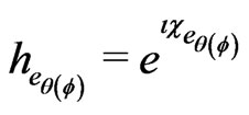 . If we plug in the actual values, we get this to be
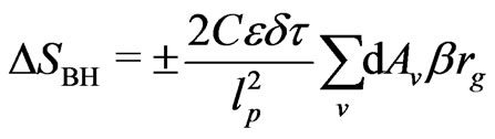 (61)
(61)
where  the area element at vertex
  on the sphere. This change in entropy is totally gravitational in origin, and seems to signify the emergence of “geometry” from within the horizon.
In fact, if we some over the area, we get the 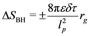 (if we set
 ), which would be the change in entropy when the radius of the horizon changes by
 !
!
4. Outgoing Flux of Radiation
In the previous section we found that as the system evolves in time, the horizon fluctuates and the area decreases. But is this Hawking radiation? Adding matter to a “coherent state” description of semiclassical gravity has been discussed [17]. Thus, given a massless scalar field Lagrangian coupled to gravity, whose Hamiltonian is given by
 (62)
(62)
the “gravity” in the Hamiltonian can be regularised in terms of the  operators in the coherent state formalism. The integral over the three volume gets converted to a sum over the vertices dotting the region. Thus
 (63)
(63)
This Hamiltonian is an operator, and one evaluates an expectation value of the Hamiltonian in the reduced density matrix of the initial slice, to find the classical behavior of the scalar field as observed by an observer outside the horizon. Thus
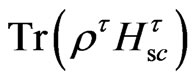 (64)
(64)
This Hamiltonian and the density matrix are then both evolved according to the time-like observers frame. One gets
 (65)
(65)
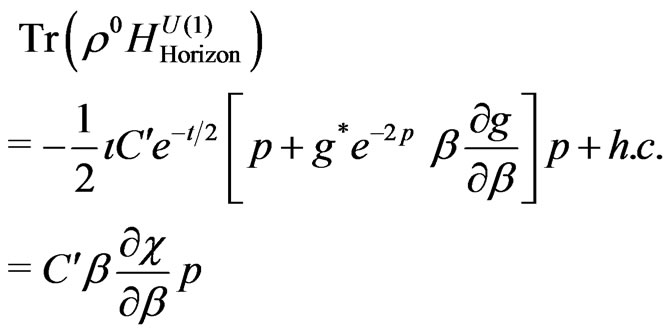
This gives
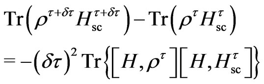 (66)
(66)
It is very clear thus that the order  terms are zero for this. However, allowing for the non-unitary evolution using the non-Hermitian Hamiltonian, the
  terms survive. In fact the terms are
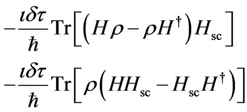 (67)
(67)
The first term is remarkable, it shows that the term giving rise to entropy change teams up with the expectation value of the scalar Hamiltonian. The second term yields corrections, so we ignore it in the first approximation. The exact details of the computation have to be obtained using the coherent state of the matter and gravity coupled system [17,18]. If one simple takes the matter + gravity system in a tensor product form, and one has matter quanta of energy  sitting at one vertex, then the first term would give new matter in the evolved slice as
 . The “rate” of particle creation thus has the form
  where
where  is the Hawking temperature for the signs
  and negative (positive)
 .
.
Thus from the above it seems 1) One has found emission of matter quanta from a black hole but from a “semiclassical” description rooted in a theory of quantum gravity, beyond quantum fields in curved space-time.
2) The results indicate a non-unitary evolution which allows space to emerge from within the horizon.
3) The emission is perceived by a static or an accelerating observer as anticipated, and the non-unitary flow might be due to the semiclassical approximations. A quantum evolution using the quantum Hamiltonian might still be unitary.
The above derivation seems to be a “quantum gravity” description of the tunneling mechanism for describing Hawking radiation [19]. However, the results are preliminary and further investigation has to be done.
5. Conclusion
In this paper we showed a method to obtain the origin of Hawking radiation using a coherent state description of a black hole space-time. We took a quantum wavefunction defined on an initial slice, peaked with maximum probability at classical phase space-variables. We then evolved the slice using a Hamiltonian, which is the “quasilocal energy” at the horizon. This QLE evolved the system in the time and the entropy was shown to change, indicating a change in black hole mass and hence an emergence of interesting non-unitary dynamics. One of course has to investigate further to see what is the endpoint of this time evolution. The time flow indicates one might have to formulate quantum theory of gravity rooted in irreversible physics. The presence of additional degrees of freedom in the form of “graphs” also indicates that the classical phase space might not be described by deterministic physics, but by distributions, a manifestation of microscopic irreversible physics in complex systems.
6. Acknowledgements
This research is supported by NSERC; research funds of University of Lethbridge. I would like to thank B. Dittrich for useful discussion; J. Supina for proofreading the manuscript.
REFERENCES
- A. Ashtekar, “New Perspectives in Canonical Gravity,” Bibliopolis, Napoli, 1988.
- C. Rovelli, “Quantum Gravity,” Cambridge University Press, Cambridge, 2004. doi:10.1017/CBO9780511755804
- T. Thiemann, “Introduction to Modern Canonical Quantum General Relativity,” Cambridge University Press, Cambridge, 2007. doi:10.1017/CBO9780511755682
- B. Hall, “The Segal-Bargmann ‘Coherent State’ Transform for Compact Lie Groups,” Journal of Functional Analysis, Vol. 122, No. 1, 1994, pp. 103-151. doi:10.1006/jfan.1994.1064
- T. Thiemann, “Gauge Field Theory Coherent States (GCS): 1. General Properties,” Classical and Quantum Gravity, Vol. 18, No. 1, 2001, pp. 2025-2064. doi:10.1088/0264-9381/18/11/304
- A. Dasgupta, “Semiclassical Quantisation of Space-Times with Apparent Horizons,” Classical and Quantum Gravity, Vol. 23, No. 3, 2006, pp. 635-671. doi:10.1088/0264-9381/23/3/007
- A. Dasgupta, “Coherent States for Black Holes,” Journal of Cosmology and Astroparticle Physics, Vol. 3, No. 8, 2004, pp. 1-36.
- A. Dasgupta, “Semiclassical Horizons,” Canadian Journal of Physics, Vol. 86, No. 4, 2008, pp. 659-662.
- A. Dasgupta and H. Thomas, “Correcting Gravitational Entropy of Spherically Symmetric Horizons,” 2006. arXiv:gr-qc/0602006
- A. Dasgupta, “Entropic Origin of Hawking Radiation,” Proceedings of 12th Marcel Grossman Meeting, Paris, July 2009.
- J. Brown and J. York, “Quasilocal Energy and Conserved Charges Derived from the Gravitational Action,” Physical Review D, Vol. 47, No. 4, 1993, pp. 1407-1419. doi:10.1103/PhysRevD.47.1407
- B. Dittrich and T. Thiemann, “Testing the Master Constraint Program for Loop Quantum Gravity: I. General Framework Class,” Classical and Quantum Gravity, Vol. 23, No. 4, 2006, pp. 1025-1066. doi:10.1088/0264-9381/23/4/001
- B. Bahr and T. Thiemann, “Gauge-Invariant Coherent States for Loop Quantum Gravity. II. Non-Abelian Gauge Groups,” Classical and Quantum Gravity, Vol. 26, No. 4, 2009, Article ID: 045012.
- A. Ashtekar, J. Baez, K. Krasnov and A. Corichi, “Quantum Geometry and Black Hole Entropy,” Physical Review Letters, Vol. 80, No. 5, 1998, pp. 904-907. doi:10.1103/PhysRevLett.80.904
- S. W. Hawking and G. Horowitz, “The Gravitational Hamiltonian, Action, Entropy and Surface Terms,” Classical and Quantum Gravity, Vol. 13, No. 6, 1996, pp. 1487- 1498. doi:10.1088/0264-9381/13/6/017
- T. Thiemann and O. Winkler, “Gauge Field Theory Coherent States (GCS) III: Ehrenfest Theorems,” Classical and Quantum Gravity, Vol. 18, No. 21, 2001, pp. 4629-46841. doi:10.1088/0264-9381/18/21/315
- H. Sahlmann and T. Thiemann, “Towards the QFT on Curved Space-Time Limit of QGR. 1. A General Scheme,” Classical and Quantum Gravity, Vol. 23, No. 3, 2006, pp. 867-908. doi:10.1088/0264-9381/23/3/019
- H. Sahlmann and T. Thiemann, “Towards the QFT on Curved Space-Time Limit of QGR. 2. A Concrete Implementation,” Classical and Quantum Gravity, Vol. 23, No. 3, 2006, pp. 909-954. doi:10.1088/0264-9381/23/3/020
- M. K. Parikh and F. Wilczek, “Hawking Radiation as Tunneling,” Physical Review Letters, Vol. 85, No. 24, 2000, pp. 5042-5045. doi:10.1103/PhysRevLett.85.5042