Applied Mathematics
Vol.5 No.13(2014), Article ID:47985,11 pages
DOI:10.4236/am.2014.513200
Wavelet Density Estimation of Censoring Data and Evaluate of Mean Integral Square Error with Convergence Ratio and Empirical Distribution of Given Estimator
Mahmoud Afshari
Department of Statistics, College of Science, Persian Gulf University, Bushehr, Iran
Email: afshar@pgu.ac.ir
Copyright © 2014 by author and Scientific Research Publishing Inc.
This work is licensed under the Creative Commons Attribution International License (CC BY).
http://creativecommons.org/licenses/by/4.0/


Received 19 April 2014; revised 29 May 2014; accepted 12 June 2014
ABSTRACT
Wavelet has rapid development in the current mathematics new areas. It also has a double meaning of theory and application. In signal and image compression, signal analysis, engineering technology has a wide range of applications. In this paper, we use wavelet method, for estimating the density function for censoring data. We evaluate the mean integrated squared error, convergence ratio of given estimator. Also, we obtain empirical distribution of given estimator and verify the conclusion by two simulation examples.
Keywords:Wavelet Estimation, Censoring, Mean Integral Error, Convergence

1. Introduction
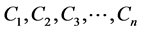
One of data types, which researchers are extremely interested in, is caring to the
time interval till the occurrence of certain events such as death etc. Any process
waiting for a specific event produces survival data. Survival function, which is
shown by , indicates the ratio of people
who survived since the base time which is the point they enter the experiment. Failure
in survival analysis means the occurrence of the event we were waiting for. The
time, where survival is measured after that point, is called the start time. The
failure time is the time that failure occurs for each individual which is denoted
by
, indicates the ratio of people
who survived since the base time which is the point they enter the experiment. Failure
in survival analysis means the occurrence of the event we were waiting for. The
time, where survival is measured after that point, is called the start time. The
failure time is the time that failure occurs for each individual which is denoted
by
 for
for . The failure time is occurred from the base time up
to when the failure occurs and it’s known as
. The failure time is occurred from the base time up
to when the failure occurs and it’s known as
 . It’s not always possible to observe the failure time
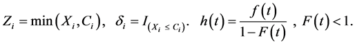
for each individual. In such cases, censorship occurs. The rate of occurrences of
an event (failure) in a specific short period of time providing that no failure
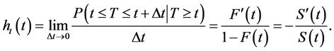
occurred before that time is the concept which is discussed by the name hazard function
in survival analysis. Hazard function for the failure time line is as follows:
. It’s not always possible to observe the failure time
for each individual. In such cases, censorship occurs. The rate of occurrences of
an event (failure) in a specific short period of time providing that no failure
occurred before that time is the concept which is discussed by the name hazard function
in survival analysis. Hazard function for the failure time line is as follows:
Wavelets can be used for transient phenomena analysis or functions analysis which sometimes changes rapidly, and they are symmetrical and have limited period unlike rugged Sine waves, thus the signals with radical changes are analyzed better. The close relationship between wavelet coefficients and some spaces, wavelet bases being orthogonal and also useful properties of them in wavelet issues simplify the computational algorithms.
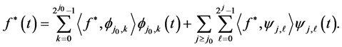
Wavelets theory was proposed by Alfred Harr [1] for the first time in 1910. He showed that a continuous function can be approximated as follows:
 (1)
(1)
Such that
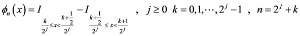
Also for mother wavelet and father wavelets the following:
Definition 1-1: Assume that ;
;
 is an orthogonal unit base for
 and
and
 contains all sectionally constant functions and their exact length is twice the
interval length of
contains all sectionally constant functions and their exact length is twice the
interval length of .
.
Spaces
 are called multiresolatio analysis or scale function
 , if it satisfies
the following conditions:
, if it satisfies
the following conditions:
1- , 2-
, 2- , 3-
, 3- 4-
4- , 5-‘
, 5-‘ .
.
6- in condition that
 is an orthogonal base for
 .
.
If we consider the scale function in the interval , then the image of f on the
space Vj is defined as
, then the image of f on the
space Vj is defined as
 which is a function with the resolution,
 and because of the fact that
thus
 is a good approximation of function
 for large amounts of
 .
.
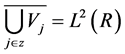
Let the nested sequence of closed subspaces; …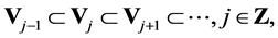 be a multiresolutuon approximation
to
be a multiresolutuon approximation
to . Define
 ,
,
 to be orthogonal complement of
 in
in .
.
The term wavelets are used to refer to a set of basis functions with very special
structure. The special of wavelets basis for function
 as scaling function
 and mother wavelet
 such that
 forms an orthogonal basis for
 and
and
 forms an orthonormal basis for
 . Other wavelets in the basis
are then generated by translation of the scaling function and dilations of the mother
wavelet by using the relationships:
. Other wavelets in the basis
are then generated by translation of the scaling function and dilations of the mother
wavelet by using the relationships:
 (2)
(2)
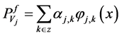
Given above Wavelet basis, a function
 can be written a formal expansion:
 (3)
(3)
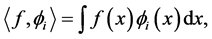
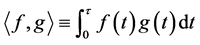
where

As for general orthogonal series estimator, Daubechies [2] , density estimator can be written as:
 (4)
(4)
where the obvious coefficient estimator can be written:
 (5)
(5)
We divide time axis into two parts, the intervals and the number of events in each interval. We determine number of events and hazard function according to the observations. Then we flatten them separately via linear wavelet density estimation on the whole time and then we calculate the function estimator and evaluate the asymptotic distribution.
In this paper we obtain estimator density for censoring data by using wavelet method and evaluate mean integral square error with convergence ratio and empirical distribution of given estimator.
2. Estimator of Density by Using Wavelet Method
Wavelets can be used for transient phenomena analysis or functions analysis which sometimes changes rapidly, and they are symmetrical and have limited period unlike rugged Sine waves, thus the signals with radical changes are analyzed better. The close relationship between wavelet coefficients and some spaces, wavelet bases being orthogonal and also useful properties of them in wavelet issues simplify the computational algorithms. As a result, numerous articles have been published about density function estimation. The mathematical theorem of wavelets and their application in statistics have been studied as a technique for nonparametric curve estimators by Antoniadys [3] .
Afshari [4] -[6] have done some researches about density function estimator, the density functional derivative and the nonparametric regression function for the mixing random variables. Donohu [7] , kyacharyan, Picard [8] , Malat [9] , Meyer [10] , and some articles have been published in this field. Hall and Patil [11] have found a formula for the Mean Integrated Squared Error of Nonlinear Wavelet based on density estimators. Antoniadys et al. [12] achieved the density function estimator and the hazard function for right-censored data with the wavelets. In this section we obtain estimator of density function for censoring data by using wavelet method.
Suppose
 are failure time of
 tests that are studied. They are non-negative, independent, identically distributed,
with the density function
tests that are studied. They are non-negative, independent, identically distributed,
with the density function
 and distribution function
 and
and
 are corresponding to censored times, non-negative, independent, identically distributed,
with the density function
are corresponding to censored times, non-negative, independent, identically distributed,
with the density function
 and distribution function
 .
.
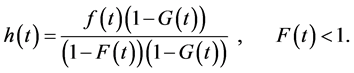
Assuming independency of failure times and censored time of the observed random
variable,
 and the function
 and Hazard function are shown as below:
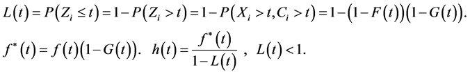
Such that
 is indicator function of
 . For data censoring,
if
. For data censoring,
if
 then we have as the following:
Also we definite as follows:
To estimate , we divide the time axis into
two parts of small intervals and the amounts of events (0 or 1) in each interval,
and then we divide these values to the length of intervals.
, we divide the time axis into
two parts of small intervals and the amounts of events (0 or 1) in each interval,
and then we divide these values to the length of intervals.
Estimation procedures of
 can be summarized as the following:
Select
 and collect the observed failures in
 intervals with the length
 and using wavelet estimation on the collected data. We find an estimate of sub density.
This means that we calculate the collected wavelet coefficients data on the scale
of
and using wavelet estimation on the collected data. We find an estimate of sub density.
This means that we calculate the collected wavelet coefficients data on the scale
of
 by choosing the decomposition level
 and then we estimate
 . It is necessary to state the
following symbols to show the details:
. It is necessary to state the
following symbols to show the details:

We figure estimators on the finite interval
 in which
 . Note that if
 is the ordinal order statistic
![]() of the sequence
of the sequence
 then
then . In fact we suppose
 .
.
Suppose that
 is an integer that could be dependent to
 and the estimated points are as follows:

Suppose that
 and we divide the interval
 of time axis to
 intervals with
 long
long
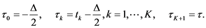
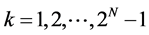
The
 -th interval is marked by
 so:
so:
 for
for .
.
Now we define the following indicator function that indicates the number of uncensored
failures in the time interval
 We assume that
 the observed failures ratio in the interval
 n other words:

Theorem 2-1: Suppose that the sub density
 is a continuous function on
 and it’s m times differentiable, then if v
 or
or , we have:
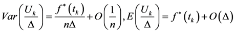

Proof: see [13] .
We smooth the data
 by an appropriate wavelet smoother to find the estimation of
 .
.
We can write,
 (6)
(6)
where,
The complex structural polymorphism analysis causes an efficient tree construction
algorithm for analysis of functions in
 with theoretic scale wavelet coefficients
 . However, the integral scale
 is not well available and we need an initial value for a fast wavelet transform.
Antonyadys [4] suggested the following initial
amount:
is not well available and we need an initial value for a fast wavelet transform.
Antonyadys [4] suggested the following initial
amount:

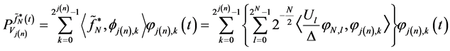
As a result a reasonable estimate for image of
 with clarity
 is:
is:
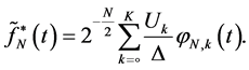 (7)
(7)
If we assume that the collected values which are equal to the estimators of
 , are in Sobolev space
 and
and
 is regular of degree
 . We estimate the
unknown function
. We estimate the
unknown function
 as follows to level the data with a better rate for the sample size
 and the sequence
 :
:
 (8)
(8)
That it is the orthogonal image of
 on the leveler approximation space
 .
.
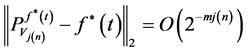
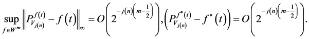
Theorem 2-2: Suppose that the sub density
 is a continuous function on
 and it’s m times differentiable, then if
 for
for
 we have:

Proof: by using theorem (2-1) we can write:
 (9)
(9)
Since,
 , then
 and we can write as the following:

So Equations (9) can be written as follows:
 (10)
(10)
By using Equation (1) we have:
 (11)
(11)
By using Equations (10) and (11) we have:


By using theorem (2-1) we can writhe as follows:
Using this fact that
 is uniformly bounded on
 and
and , we have:
 (12)
(12)
Since
 is regular in order
 we can write:
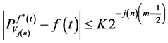
 (13)
(13)
According Equation (13), we can write: , complete the proof.
3. Evaluate of Mean Integral Square Error with Convergence Ratio
In this section we evaluate mean integral square error and convergence ratio is investigated.
Definition 3-1: The mean integrated square error (MISE) of kernel estimator of a
density function
 is given
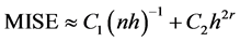 . In this formula
 denotes the right and left convergence, when
 ,
,
 denotes the sample size,
 denotes the estimator bandwidth core,
 denotes core level and
 ,
,
 denote kernel dependent quantities with unknown density.
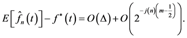
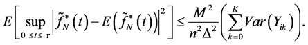
Theorem 3-1: Suppose that the sub density
 is a continuous function on
 and it’s
 times differentiable, then if
 for
for
 and
and , then
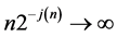 ,
,
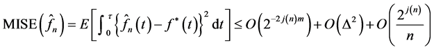 (14)
(14)
Proof:
 (15)
(15)
By using Equation (15) and theorem (2-2) for , we can write as
the following:
, we can write as
the following:

Because
 we can write as the following:
 (16)
(16)
 (17)
(17)
So by using Equations (16) and (17), we can write:
 (18)
(18)
For evaluate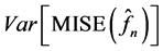 , we can write:
Also we can write:
 then,
then,
 (19)
(19)
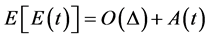
By using theorem (2-1) and expectation of Equation (19), we can write as the following:
 (20)
(20)
By using theorem (2-1) we have:
 (21)
(21)
 (22)
(22)
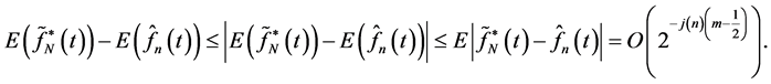
By using Equation (22) and this fact that
 is uniformly bounded, we can write as the following:
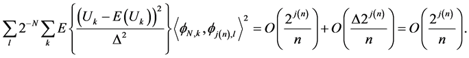
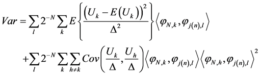
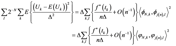
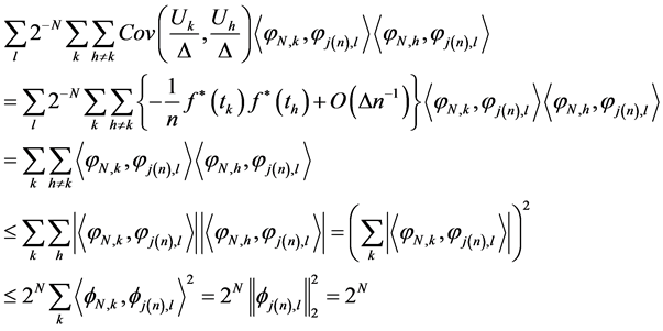
The second part of Equation (20) can be written as the following:
By using , the proof is complete.
4. Empirical Distribution of Purpose Estimator
In this section we investigate empirical distribution of estimator under some condition.
Theorem 4-1 Suppose that the sub density
 is a continuous function on
 and it’s m times differentiable, for
 ,
,
 ,
,
 ,
,
 , then for interval
 , we have:
 .
.
Proof:

By using theorems (2-1) and (2-2), we can write as the following:
 (23)
(23)
 (24)
(24)
So by using equation of (23) and (24) we can write as the following:
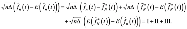
We prove that II has asymptotically normal distribution and also I, III tend to
zero when

First, we show that I, III tend to zero when . According to Equation
(24) we have:
. According to Equation
(24) we have:
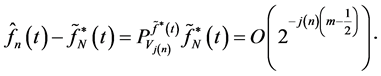
 (25)
(25)
By using Equation (23) we have:
 .
.
So by using Equation (24) and (25), the phrase I, III tend to zero when , and finally we
have:
, and finally we
have:
So we have:
 (26)
(26)
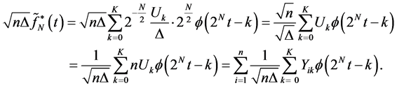
Such that for each fixed , while
 ,
,
 is defined as an independent and identically distributed
random sample with the mean as follows:
is defined as an independent and identically distributed
random sample with the mean as follows:

By using cushy Schwartz inequality:
 (27)
(27)
So we can write as the following:
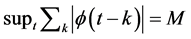
Using this fact that
 is uniformly bounded and,
 ,
,
 , we can write:
 ,
,

Thus, the Equation (26) state is convergent in
 and thus in the distribution.
Also by using Theorem (2-2), we have:
Thus we have:
We control the Lindberg condition in order to prove that II is asymptotically normal.
For this purpose, we set:
 and we show that
By using cushy Schwartz inequality:
 , So we can write as the following:
 and complete the proof.
5. Simulation and Numerical Computation for Target Estimator
In this section we simulate,
 on the data of size
 by using Semlayt’s wavelet. We consider convergence ratio of given estimator by
computing of average mean square error of given estimators. We use
by using Semlayt’s wavelet. We consider convergence ratio of given estimator by
computing of average mean square error of given estimators. We use
 software and wavelet package for simulation.
Example 1: We generate
 and
and
 from the Samples of size
 and
and
 with
with ,
,
 ,
,
 and
and
 for optimal surface
 .
.
The results in Table 1 displays the average mean
square errors of subdensity function estimator for sample sizes
 and
and .
.
The panel in Figure 1 displays the wavelet estimator
of subdensity
 of observed failures for a traditional censoring data. The solid line is the density
estimator and the dotted line is the true density.
of observed failures for a traditional censoring data. The solid line is the density
estimator and the dotted line is the true density.
Example 2: Suppose that , where
 and
and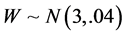 . We generate
 from sample size of
 and
and
 with
with ,
,
 ,
,
 and
and .
.
The results in Table 2 displays the average mean
square errors of subdensity function estimator for sample sizes
 and
and .
.
The panel in Figure 2 displays the wavelet estimator of subdensity of observed failures for a traditional censoring data. The solid line displays the subdensity estimates based actual data and the dotted line is the true density.

Table 1. The average mean square errors of subdensity function estimator by wavelet method.
Table 2. The average mean square errors of subdensity function estimator by wavelet method.
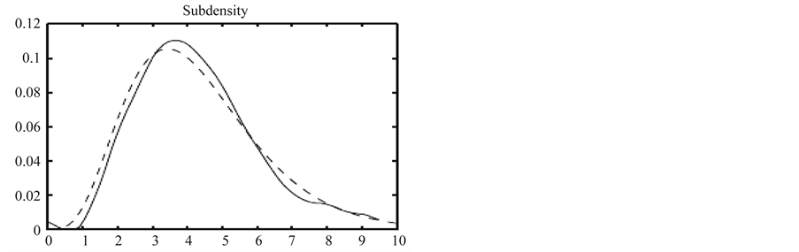
Figure 1. The wavelet subdensity and true density estimator.
Figure 2. The wavelet subdensity and true density estimator.
6. Conclusion
In this paper we obtain density estimation for censoring data by using wavelet method and evaluate mean integral square error. We show that convergence ratio is acceptable and empirical distribution of given estimator under some condition is normal.
Acknowledgements
The support of Research Committee of Persian Gulf University is greatly acknowledged.
References
- Harr, A. (1910) Zur Theorie der Orthogonalen Funktionen. Mathematische Annalen, 69, 331-371.
- Daubechies, I. (1988) Orthogonal Bases of Compactly Supported Wavelets. Communication in Pure and Applied Mathematics, 41, 909-996.
- Antoniadis, A. (1996) Smoothing Noisy Data with Tapered Coiflets Series. Scandinavian Journal of Statistics, 23, 313-330.
- Afshari, M. (2013) A Fast Wavelet Algorithm for Analyzing of Signal Processing and Empirical Distribution of Wavelet Coefficients with Numerical Example and Simulation. Communication of Statistics-Theory and Methods, 42, 4156-4169.
- Afshari, M. (2014) Estimation of Hazard Function for Censoring Random Variable by Using Wavelet Decomposition and Evaluate of MISE, AMSE With Simulation. Journal of Data Analysis and Information Processing, 2, 1-5. http://dx.doi.org/10.4236/jdaip.2014.21001
- Afshari, M. (2008) Wavelet-Kernel Estimation of Regression Function for Uniformly Mixing Process. Word Applied Sciences Journal, 4, 605-609.
- Donoha, D.L. and Johnstone, I.M. (1994) Ideal Spatial Adaptation by Wavelet Shrinkage. Biometrika Journal, 81, 425-455. http://dx.doi.org/10.1093/biomet/81.3.425
- Kerkyacharian, G. and Picard, D. (1993) Density Estimation Bykernel and Probability. McGraw-Hill Science, New York, 327-336.
- Mallat, S.G. (1989) A Theory for Multiresolution Signal Decomposition: The Wavelet Representation. Transformations on Pattern Analysis and Machine Intelligence, 11, 674-693.
- Meyer, Y. (1990) On de lettes et operateurs. Hermann, Paris.
- Hall, P. and Patil, P. (1995) Formula for Mean Integrated Squarederror of Non-Linear Wavelet Based Density Estimators. Annals of Statistics, 23, 905-928. http://dx.doi.org/10.1214/aos/1176324628
- Antoniadis, A., Gregoire, G. and Nason, P. (1999) Density and Hazard Rate Estimation for Right Censored Data Using Wavelet Methods. Journal of Royal Statistical Society Series B, 23, 313-330.
- Vidakovik, B. (1999) Statistical Modeling by Wavelets. Wiley, New York. http://dx.doi.org/10.1002/9780470317020