Applied Mathematics
Vol.4 No.8A(2013), Article ID:35481,7 pages DOI:10.4236/am.2013.48A023
Immune Control of Equine Infectious Anemia Virus Infection by Cell-Mediated and Humoral Responses
1Department of Mathematics, Washington State University, Pullman, WA, USA
2School of Biological Sciences, Washington State University, Pullman, WA, USA
3Department of Mathematics and Computational Science, University of South Carolina Beaufort, Bluffton, SC, USA
Email: *ejs@wsu.edu
Copyright © 2013 Elissa J. Schwartz et al. This is an open access article distributed under the Creative Commons Attribution License, which permits unrestricted use, distribution, and reproduction in any medium, provided the original work is properly cited.
Received June 3, 2013; revised July 3, 2013; accepted July 10, 2013
Keywords: Deterministic Model; Virus Infection; Equine Infectious Anemia Virus; Immune Response; Antibodies; Cytotoxic T Lymphocytes
ABSTRACT
Equine Infectious Anemia Virus (EIAV) is a retrovirus that establishes a persistent infection in horses and ponies. The virus is in the same lentivirus subgroup that includes human immunodeficiency virus (HIV). The similarities between these two viruses make the study of the immune response to EIAV relevant to research on HIV. We developed a mathematical model of within-host EIAV infection dynamics that contains both humoral and cell-mediated immune responses. Analysis of the model yields results on thresholds that would be necessary for a combined immune response to successfully control infection. Numerical simulations are presented to illustrate the results. These findings have the potential to lead to immunological control measures for lentiviral infection.
1. Introduction
One of the most significant gaps in our knowledge of virus-host dynamics involves how different immune responses work together to counteract the pathogen. Understanding viral dynamics in the context of immune responses is essential for advancing our knowledge of host-pathogen interactions as well as for developing control strategies. Mathematical modeling has been instrumental in the study of viral dynamics and has increased our understanding of basic pathogenic interactions for infections including human immunodeficiency virus, hepatitis B virus, hepatitis C virus, and influenza virus [1-6]. In this paper, we study Equine Infectious Anemia Virus (EIAV).
EIAV is a retrovirus of the genus lentivirus that infects equids such as horses and ponies. EIAV is spread between horses through biting flies [7]. Horse flies, primarily of the family Tabanidae [8], feed on acutely infected horses and spread the virus through a subsequent blood meal on an uninfected equid. Due to this insect vector, EIAV tends to be concentrated in warmer climates, but is considered a worldwide infection [7,9]. To control the spread of infection, horses are routinely tested at racetracks, shows, and rodeos, before breeding, and crossing borders. This effort has proven largely successful, bringing the prevalence of EIAV-positive animals down to 0.38% by 1988 [7,10].
EIAV targets monocyte-derived macrophages in several tissues of infected equids, including spleen, liver, lungs, and bone marrow [7,11]. These tissues serve as reservoirs for infection for the remainder of the animal’s life. Immune control of EIAV is attributed to both cytotoxic T lymphocyte (CTL) [12,13] and broadly neutralizing antibody (bnAb) [14] activity. Due to the changing dynamics of both the CTL and bnAb responses in both specificity and timing, it is believed that both responses are essential for long-term control of the infection.
Infection with EIAV typically follows three stages: acute, chronic, and asymptomatic [7]. The acute stage is an initial febrile episode associated with the onset of infection, high viral titer, and an adaptive immune response. Once the initial infection is brought under control, antigenic variants escape the immunological control and cause the increases in viral load and fevers associated with the chronic stage. After six to twelve months, the recurrent fevers cease and the animal enters the asymptomatic stage, which is associated with very low viral load and the absence of clinical symptoms. In some cases, a fourth recrudescent stage is seen, where the infected animal experiences recurring fevers for the remainder of its life. This stage is often associated with immunosuppressed or otherwise immunocompromised animals [15].
EIAV shows many life history traits similar to other lentiviruses, including a very rapid replication rate and high levels of antigenic variation. However, EIAV is atypical among lentiviruses in that most infected animals experience a few episodes of fever and high viral titer and then progress to the asymptomatic stage characterized by low viral titer and an absence of clinical disease manifestations. This is in direct contrast to lentiviruses human immunodeficiency virus (HIV) and simian immunodeficiency virus (SIV), in which infected individuals and animals develop immunodeficiency and disease, and makes EIAV an especially interesting comparison species for both clinical research and mathematical models [16].
There is a great body of previous work modeling the dynamics of viral infection. The standard three equation model of viral infection considers the uninfected cell, infected cell, and virus populations but does not include the dynamics of immune compartments [16-18]. Subsequent models augmented the standard model to four or five equations, examining the dynamics of the cellular (CTL) and humoral (antibody) immune responses individually [17,19] and in concert [20]. Two studies explicitly modeled viral dynamics with the dynamics of CTLs and antibodies to study Hepatitis C Virus (HCV) [21,22]. Wodarz investigated the dynamics and pathology of HCV, and Yousfi et al. extended the theoretical results by Wodarz with a global stability analysis. However, these studies used a model with a depiction of antibody production in which antibodies proliferate according to mass action between antibodies and virus; this depiction is imprecise and a more accurate representation is needed.
The goal of this study is to create a mathematical model of EIAV and immune system dynamics in order to predict conditions that correlate with viral control. We use a five-equation model, explicitly containing the dynamics of CTLs and of antibodies, which builds upon previous work. We include an alternate equation for antibody dynamics that models antibody production in direct proportion to virus, consistent with known immunology [23]. We use our model to gain insight into EIAV infection, in which both CTL and antibody responses are known to be important for control. Specifically, our analysis gives the characteristics of 3 scenarios: no infection, viral persistence without CTLs, and viral persistence with both CTL and antibody responses. We simulate the longterm dynamics of viral infection, showing viral persistence in the context of antibodies alone or of both antibodies and CTLs.
This paper is organized as follows: Section 2 contains a description of the deterministic model along with its equilibrium points. In Section 3 we discuss the linear stability analysis of the biologically relevant equilibria and the conditions for their stability. In addition we discuss the basic reproduction number,  , of the model. We also provide numerical simulations that illustrate the behavior of solutions for representative parameter sets. In Section 4 we conclude the paper with a discussion of the implications of these results for understanding control of EIAV infection by the cell-mediated and humoral arms of the immune response.
2. Mathematical Model
In this section we present a five-equation model that builds upon earlier studies [16,17,21,22]. Our model explicitly contains the dynamics of CTLs and antibodies, including an equation for antibody dynamics that models antibody production in direct proportion to virus [23]. We then find the steady state solutions.
2.1. Model Formulation
Our deterministic model representing the five interacting populations is shown by the following system of ordinary differential equations:
In this model, the target cells of EIAV infection are monocyte-derived tissue macrophages [7,11,24,25]. The number of uninfected target cells is represented by M. These cells become infected cells (I) following contact with virus (V) at rate . Uninfected target cells are generated at rate
 ![]() and die at rate
and die at rate . The infected cell death rate is
![]() . Infected cells are killed by cytotoxic T lymphocytes, or CTLs (C), at rate
. Infected cells are killed by cytotoxic T lymphocytes, or CTLs (C), at rate . Virus is produced by infected cells at rate b and cleared at rate γ. The virus is neutralized by antibodies (A) at rate
 . CTLs proliferate in response to contact with infected cells at rate
  and die at rate
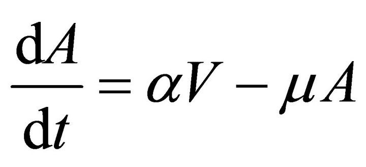
![]() . The antibody population grows in proportion to virus at rate α [23] and is cleared at rate
. The antibody population grows in proportion to virus at rate α [23] and is cleared at rate . A schematic diagram of the model dynamics, indicating the flow in and out of each compartment, is shown in Figure 1. Model variables and parameters are listed in Table 1. The initial conditions for the model are
  and
and 
 . We assume all parameters are nonnegative.
2.2. Equilibrium Points
The equilibria (or steady states) of the model are found by setting the equations of the model to zero. The infection-free steady state (also called the infection-free equilibrium, or IFE) is given by
We obtain four other solutions: and
and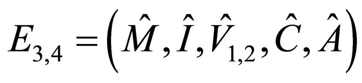 , where
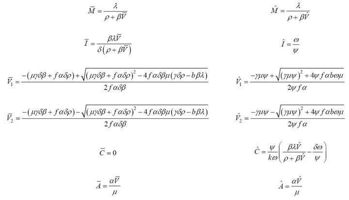
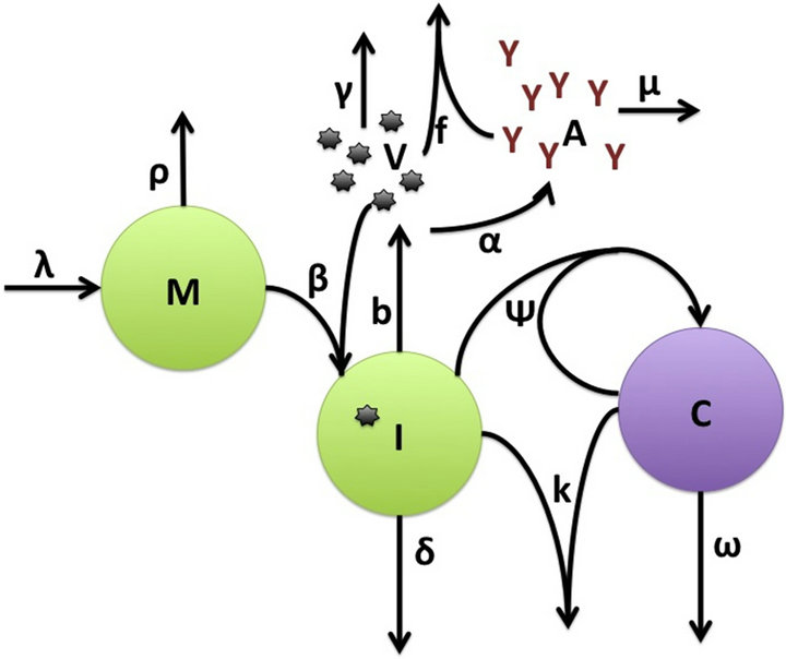
Figure 1. Schematic diagram of mathematical model of EIAV infection with cellular and humoral immune responses. Populations modeled include the target cells (macrophages, M), infected cells (I), virus (V), cytotoxic T lymphocytes (C) and antibodies (A).
Table 1. Parameters and variables of model of EIAV infection.
Since  and
and  are less than zero, the steady states
  and
and  are not biologically meaningful and therefore will not be discussed further.
3. Linear Stability Analysis of Model Equilibria
In this section we discuss the basic reproductive number,  , which arises from linear analysis around the infection-free equilibrium point,
 . We provide stability conditions for
  in Theorem 2, and we provide existence criteria for
  and
and  in Theorem 3. In addition we provide a numerical stability analysis as well as numerical simulations that illustrate the stability of these equilibrium points.
3.1. Analytical Results
The basic reproductive number,  , is a threshold that delineates whether an infection spreads or dies out when a single infected cell encounters a population of uninfected target cells [26-30]. If
 , then more than one cell (on average) becomes infected and the infection will spread; if
 , then less than one cell (on average) becomes infected and infection will not take hold [31].
Theorem 1. The basic reproductive number of the model is .
.
Proof. We determine  using the next-generation method [32]. Consider the matrix of new infections,
  , and the matrix of transfers,
  , both evaluated at the infection-free equilibrium:
 and
and . Hence,
 .
.
The basic reproductive number is given by the spectral radius (i.e., the eigenvalue with the largest modulus) of
 . Hence,
 .
.
Theorem 2. The IFE,  , of the model is linearly asymptotically stable and attracting for
  and unstable for
 .
.
Proof. That the IFE is linearly asymptotically stable and attracting for  but unstable for
  is an immediate consequence of the computations provided in Theorem 1 and the results of van den Driessche and Watmough [32].
The equilibrium  exists if
  is biologically relevant, i.e.,
 .
.  can be rewritten as
 , where
 . Hence,
  exists if
 .
.
We will refer to  as the boundary equilibrium, which represents the case with the presence of antibodies and without CTLs. We will refer to
  as the endemic equilibrium, which represents the case with the presence of both antibodies and CTLs.
Theorem 3. If , then
  is the only equilibrium point and is linearly stable. If
 , then
  is unstable, and boundary equilibrium
  exists. If
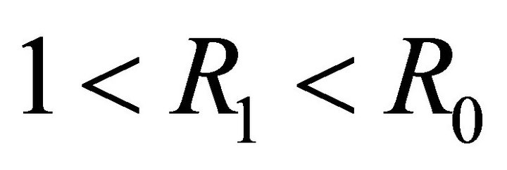 , then
  is unstable, boundary equilibrium
  exists, and endemic equilibrium
  exists.
Proof. We obtain that  from the inequalities
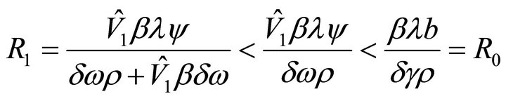
since . The latter inequality is shown as follows.
In determining the equilibrium points  and
and , the values
  and
and  were found as the roots of the quadratic function
 .
.
Since the leading coefficient of  is positiveand
 , then the positive root
  lies to the left of the positive value
 . That is,
 .
.
We now consider the existence of the equilibrium points  and
and . This is determined by the sign of the roots
  and
and  of the quadratic function
 .
.
Since , then if
 , we obtain
which implies that  and
and . Hence, the equilibrium points
  and
and  are not biologically possible. If
 , we obtain

which implies that  and
and . This indicates that
  is an existing equilibrium.
The endemic equilibrium  exists only if
 .
.
Since ,
,  is biologically possible only if
 . Theorem 3 follows from the arguments above.
We note that  is a threshold that delineates the boundary equilibrium
  from the endemic equilibrium
 .
.
3.2. Numerical Stability Analysis
In the previous sections we found the steady states of the model and determined thresholds for their linear stability. The biologically plausible steady states ,
,  , and
, and  represent the scenarios of the infection-free equilibrium (IFE), the boundary equilibrium with no CTLs, and the endemic equilibrium with both CTL and antibody function (Ab), respectively.
We next performed a linear stability analysis of the equilibria of the model by using numerical values for the parameters (i.e., a unique parameter set representing each of the three equilibria) and determining the eigenvalues of the Jacobian matrices evaluated at each steady state. Negative real parts of all the eigenvalues indicated stability of the steady state. We present the results using three representative parameter sets. Our results are summarized in Table 2. Parameter sets 1, 2, and 3 were selected because they predict equilibria ,
,  , and
, and , respectively. These parameter sets differ in the value for λ; equivalent results were found by altering the other parameters that affect
  (data not shown).
3.3. Numerical Simulations
We now illustrate the results on linear stability with numerical simulations using each of the three parameter sets.
Infection-Free Equilibrium, E0. In the IFE, the infection dies out. All populations approach zero except the number of uninfected cells, which approaches its uninfected steady state level. The time course of infection showing each of the populations over 150 days is shown in Figure 2.
Boundary Equilibrium, E1. The boundary equilibrium  represents the case with antibodies but no CTLs. Here
  and
and . The long-term dynamics show that all populations reach a positive steady state except CTLs, which decay to zero. The time course of infection showing each of the populations over 150 days is shown in Figure 3.
Endemic Equilibrium, E3. The endemic equilibrium  shows the case with both antibodies and CTLs. We observe nonnegative steady state values for all populations. In this case,
  and
and . The time course of infection, showing each of the populations over 150 days, is shown in Figure 4. This is the case that correlates with clinical infection of horses with EIAV.
Long-term dynamics over 3000 days. Equilibrium values are seen clearly in simulations run over 3000 days. The boundary equilibrium over 3000 days is shown in Figure 5. The endemic equilibrium over 3000 days is shown in Figure 6. We observe that final values for ,
,  ,
,  and
and  are greater in
  than in
 , but this is likely due to the larger value for
 ![]() in this parameter set. For parameter set 1 representing the IFE, all populations except
in this parameter set. For parameter set 1 representing the IFE, all populations except  reach zero over 3000 days (data not shown).
4. Discussion
In summary, we constructed a mathematical model of EIAV infection that takes into account the dynamics of cell-mediated and humoral immune responses. Both of these immune components have been found to be necessary for immune control of this infection. We performed linear stability analysis and simulation of the model to predict long-term behavior in healthy and infected states. We presented equations for the basic reproductive number  as well as a second threshold,
 . We showed that
  distinguishes the IFE
  from the boundary equilibrium
  and the endemic equilibrium
 , and that
  distinguishes
  from
from . Finally, we presented parameter sets that correlate with the results of the linear stability analysis.
The steady states each describe a scenario with a different virological and immunological profile: viral clearance , control of infection with antibodies and no CTLs
 , and control of infection with both antibodies and CTLs
 . Biologically, two of these scenarios are seen in horses: viral clearance (i.e., no infection)
  and control of infection with both antibodies and CTLs (i.e., coexistence of all five populations)
 . Since coexistence is what is observed in clinical EIAV infection, knowledge of the characteristics of this steady state may be useful both for understanding fundamental mechanisms of immune control as well as for developing therapeutic strategies to bring about the control of viral
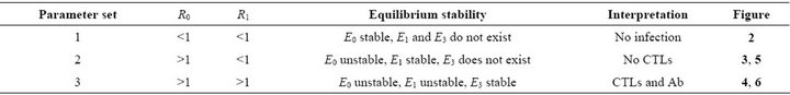
Table 2. Numerical results of linear stability analysis.
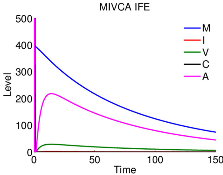
Figure 2. Long-term dynamics of M, I, V, C, and A populations over 150 days for a parameter set representing the infection-free equilibrium (IFE). Parameters are as follows: λ = 0.05, ρ = 0.01, β = 0.0001, δ = 0.5, k = 0.01, b = 10000, γ = 20, ψ = 0.75, ω = 5, f = 3, α = 150, μ = 20 (parameter set 1). Here, R0 = 0.5 and R1 = 0.
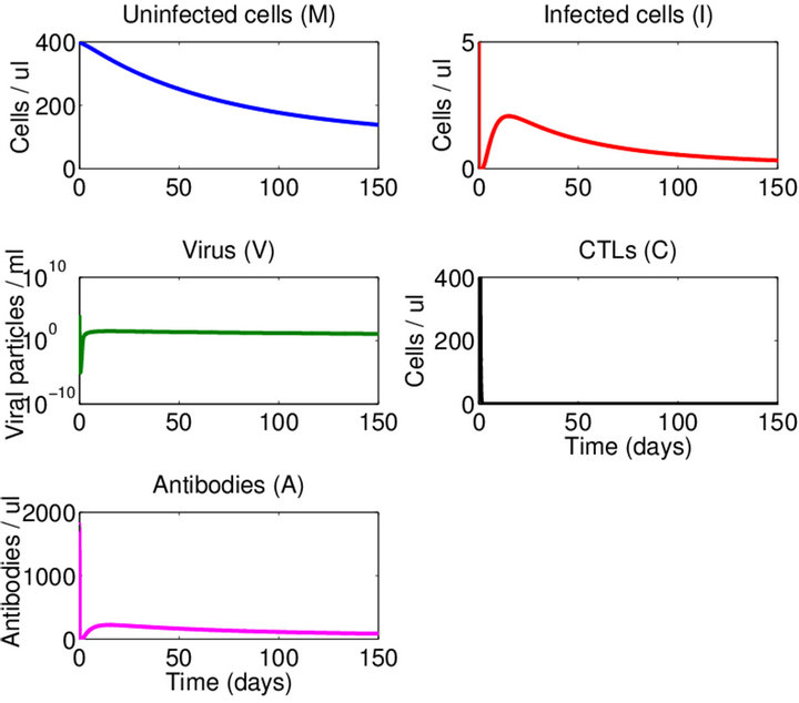
Figure 3. Long-term dynamics of M, I, V, C, and A populations over 150 days for a parameter set representing the E1 boundary equilibrium. Parameters are as in Figure 2 except λ = 1 (parameter set 2). Here, R0 = 10 and R1 = 0.02.
Figure 4. Long-term dynamics of M, I, V, C, and A populations over 150 days for a parameter set representing the E3 endemic equilibrium. Parameters are as in Figure 2 except λ = 50 (parameter set 3). Here, R0 = 500 and R1 = 5.26.
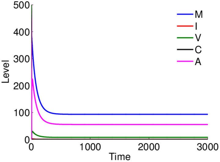
Figure 5. Long-term dynamics of M, I, V, C, and A populations over 3000 days for parameter set 2 representing the E1 boundary equilibrium. Parameters are as in Figure 3.
Figure 6. Long-term dynamics of M, I, V, C, and A populations over 3000 days for parameter set 3 representing the E3 endemic equilibrium. Parameters are as in Figure 4.
infection without disease. Future work in this area may be applicable for understanding other lentiviral infections that cause disease, such as HIV.
5. Acknowledgements
The authors would like to thank Pauline van den Driessche for insightful comments on the manuscript.
REFERENCES
- S. M. Ciupe, et al., “Modeling the Mechanisms of Acute Hepatitis B Virus Infection,” Journal of Theoretical Biology, Vol. 247, No. 1, 2007, pp. 23-35. doi:10.1016/j.jtbi.2007.02.017
- H. Dahari, et al., “The Extrahepatic Contribution to HCV Plasma Viremia,” Journal of Hepatology, Vol. 45, No. 4, 2006, pp. 626-627. doi:10.1016/j.jhep.2006.07.004
- D. D. Ho, et al., “Rapid Turnover of Plasma Virions and CD4 Lymphocytes in HIV-1 Infection,” Nature, Vol. 373, No. 6510, 1995, pp. 123-126. doi:10.1038/373123a0
- A. U. Neumann, et al., “Hepatitis C Viral Dynamics in Vivo and the Antiviral Efficacy of Interferon-Alpha Therapy,” Science, Vol. 282, No. 5386, 1998, pp. 103-107. doi:10.1126/science.282.5386.103
- X. Wei, et al., “Viral Dynamics in Human Immunodeficiency Virus Type 1 Infection,” Nature, Vol. 373, No. 6510, 1995, pp. 117-122. doi:10.1038/373117a0
- K. A. Pawelek, et al., “Modeling Within-Host Dynamics of Influenza Virus Infection Including Immune Responses,” PLoS Computational Biology, Vol. 8, No. 6, 2012, Article ID: e1002588. doi:10.1371/journal.pcbi.1002588
- C. Leroux, J. L. Cadore and R. C. Montelaro, “Equine Infectious Anemia Virus (EIAV): What Has HIV’s Country Cousin Got to Tell Us?” Veterinary Research, Vol. 35, No. 4, 2004, pp. 485-512. doi:10.1051/vetres:2004020
- E. W. Cupp and M. J. Kemen, “The Role of Stable Flies and Mosquitoes in the Transmission of Equine Infectious Anemia Virus,” Proceedings of the Annual Meeting of the United States Animal Health Association, Vol. 84, 1980, pp. 362-367.
- C. J. Issel and L. D. Foil, “Studies on Equine Infectious Anemia Virus Transmission by Insects,” Journal of the American Veterinary Medical Association, Vol. 184, No. 3, 1984, pp. 293-297.
- J. E. Pearson and C. A. Gipson, “Standardization of Equine Infectious-Anemia Immunodiffusion and Celisa Tests and Their Application to Control of the Disease in the UnitedStates,” Journal of Equine Veterinary Science, Vol. 8, No. 1, 1988, pp. 60-61. doi:10.1016/S0737-0806(88)80113-8
- B. Zhang, et al., “Mapping of Equine Lentivirus Receptor 1 Residues Critical for Equine Infectious Anemia Virus Envelope Binding,” Journal of Virology, Vol. 82, No. 3, 2008, pp. 1204-1213. doi:10.1128/JVI.01393-07
- C. Chung, R. H. Mealey and T. C. McGuire, “CTL from EIAV Carrier Horses with Diverse MHC Class I Alleles Recognize Epitope Clusters in Gag Matrix and Capsid Proteins,” Virology, Vol. 327, No. 1, 2004, pp. 144-154. doi:10.1016/j.virol.2004.06.035
- R. H. Mealey, et al., “Early Detection of Dominant EnvSpecific and Subdominant Gag-Specific CD8+ Lymphocytes in Equine Infectious Anemia Virus-Infected Horses Using Major Histocompatibility Complex Class I/Peptide Tetrameric Complexes,” Virology, Vol. 339, No. 1, 2005, pp. 110-126. doi:10.1016/j.virol.2005.05.025
- S. D. Taylor, et al., “Protective Effects of Broadly Neutralizing Immunoglobulin against Homologous and Heterologous Equine Infectious Anemia Virus Infection in Horses with Severe Combined Immunodeficiency,” Journal of Virology, Vol. 85, No. 13, 2011, pp. 6814-6818. doi:10.1128/JVI.00077-11
- Y. Kono, et al., “Recrudescence of Equine Infectious Anemia by Treatment with Immunosuppressive Drugs,” National Institute of Animal Health Quarterly (Tokyo), Vol. 16, No. 1, 1976, pp. 8-15.
- A. S. Perelson, “Modelling Viral and Immune System Dynamics,” Nature Reviews Immunology, Vol. 2, No. 1, 2002, pp. 28-36. doi:10.1038/nri700
- M. A. Nowak and C. R. Bangham, “Population Dynamics of Immune Responses to Persistent Viruses,” Science, Vol. 272, No. 5258, 1996, pp. 74-79. doi:10.1126/science.272.5258.74
- A. S. Perelson, et al., “HIV-1 Dynamics in Vivo: Virion Clearance Rate, Infected Cell Life-Span, and Viral Generation Time,” Science, Vol. 271, No. 5255, 1996, pp. 1582-1586. doi:10.1126/science.271.5255.1582
- S. M. Ciupe, P. De Leenheer and T. B. Kepler, “Paradoxical Suppression of Poly-Specific Broadly Neutralizing Antibodies in the Presence of Strain-Specific Neutralizing Antibodies Following HIV Infection,” Journal of Theoretical Biology, Vol. 277, No. 1, 2011, pp. 55-66. doi:10.1016/j.jtbi.2011.01.050
- R. Antia, S. S. Pilyugin and R. Ahmed, “Models of Immune Memory: On the Role of Cross-Reactive Stimulation, Competition, and Homeostasis in Maintaining Immune Memory,” Proceedings of the National Academy of Sciences of the USA, Vol. 95, No. 25, 1998, pp. 14926- 14931. doi:10.1073/pnas.95.25.14926
- D. Wodarz, “Hepatitis C Virus Dynamics and Pathology: The Role of CTL and Antibody Responses,” The Journal of General Virology, Vol. 84, 2003, pp. 1743-1750. doi:10.1099/vir.0.19118-0
- N. Yousfi, K. Hattaf and M. Rachik, “Analysis of a HCV Model with CTL and Antibody Responses,” Applied Mathematical Sciences, Vol. 3, No. 57, 2009, pp. 2835-2846.
- C. Janeway, “Immunobiology: The Immune System in Health and Disease,” 6th Edition, Garland Science, New York, 2005, 823 p.
- S. M. Harrold, et al., “Tissue Sites of Persistent Infection and Active Replication of Equine Infectious Anemia Virus during Acute Disease and Asymptomatic Infection in Experimentally Infected Equids,” Journal of Virology, Vol. 74, No. 7, 2000, pp. 3112-3121. doi:10.1128/JVI.74.7.3112-3121.2000
- J. L. Oaks, et al., “Equine Infectious Anemia Virus Is Found in Tissue Macrophages during Subclinical Infection,” Journal of Virology, Vol. 72, No. 9, 1998, pp. 7263- 7269.
- R. M. Anderson and R. M. May, “Infectious Diseases of Humans: Dynamics and Control,” Oxford University Press, Oxford, 1991.
- S. Bonhoeffer, et al., “Virus Dynamics and Drug Therapy,” Proceedings of the National Academy of Sciences of the USA, Vol. 94, No. 13, 1997, pp. 6971-6976. doi:10.1073/pnas.94.13.6971
- D. D. Ho and Y. Huang, “The HIV-1 Vaccine Race,” Cell, Vol. 110, No. 2, 2002, pp. 135-138. doi:10.1016/S0092-8674(02)00832-2
- S. J. Little, et al., “Viral Dynamics of Acute HIV-1 Infection,” The Journal of Experimental Medicine, Vol. 190, No. 6, 1999, pp. 841-850. doi:10.1084/jem.190.6.841
- D. Wodarz, “On the Relative Fitness of Early and Late Stage Simian Immunodeficiency Virus Isolates,” Theoretical Population Biology, Vol. 72, No. 3, 2007, pp. 426- 435. doi:10.1016/j.tpb.2007.03.005
- R. M. Ribeiro, et al., “Estimation of the Initial Viral Growth Rate and Basic Reproductive Number during Acute HIV- 1 Infection,” Journal of Virology, Vol. 84, No. 12, 2010, pp. 6096-6102. doi:10.1128/JVI.00127-10
- P. van den Driessche and J. Watmough, “Reproduction Numbers and Sub-Threshold Endemic Equilibria for Compartmental Models of Disease Transmission,” Mathematical Biosciences, Vol. 180, No. 1-2, 2002, pp. 29-48. doi:10.1016/S0025-5564(02)00108-6
NOTES
*Corresponding author.