ABSTRACT

A family of tests for the presence of regression effect under proportional and non-proportional hazards models is described. The non-proportional hazards model, although not completely general, is very broad and includes a large number of possibilities. In the absence of restrictions, the regression coefficient, , can be any real function of time. When we recover the proportional hazards model which can then be taken as a special case of a non-proportional hazards model. We study tests of the null hypothesis; for all t against alternatives such as; or for some t. In contrast to now classical approaches based on partial likelihood and martingale theory, the development here is based on Brownian motion, Donsker’s theorem and theorems from O’Quigley [1] and Xu and O’Quigley [2]. The usual partial likelihood score test arises as a special case. Large sample theory follows without special arguments, such as the martingale central limit theorem, and is relatively straightforward.

1. Introduction

1.1. Background

The complex nature of data arising in the context of survival studies is such that it is common to make use of a multivariate regression model. Cox’s semi-parametric proportional hazards model [3] has enjoyed wide use in view of its broad applicability. The model makes the key assumption that the regression coefficients do not change with time and much study has gone into investigating and correcting for potential departures from these assumptions [4-10]. Sometimes we can anticipate in advance that the proportional hazards model may be too restrictive. The example which gave rise to our own interest in this question concerned 2174 breast cancer patients, followed over a period of 15 years at the Institut Curie in Paris, France. For these data, as well as a number of other studies in breast cancer, the presence of non-proportional hazards effects has been observed by several authors. Often this is ignored but this can seriously impact inferences.

The model used to make inferences will then often differ from that which can be assumed to have generated the observations. In situations of non proportional hazards, unless dealing with very large data sets relative to the number of studied covariates, it will often not be feasible to study the whole, possibly of infinite dimension,. Xu and O’Quigley [11] argue that an estimate of average effect can be used in a preliminary analysis of a data set with time varying regression effects. For a given sample, a single average effect can be estimated more accurately (and more easily) than the whole. Xu and O’Quigley [11] derive an estimate of an average regression effect. They provide an interpretation of as a population average effect. It is approximated by under certain conditions, where F is the marginal distribution function of the failure time random variable T. The purpose here is to test the null hypothesis; for all t against the alternatives or for some t. The development is based on Brownian motion, Donsker’s theorem and theorems from O’Quigley [1] and Xu and O’Quigley [2]. We show that the usual partial likelyhood score test arises as a special case. Large sample theory is straightforward.

1.2. Notation

The probability structure, although quite simple, is not the immediate one which would come to mind. The random variables of interest are the failure time, , the censoring time, and the possibly time dependent covariate, , We view these as a random sample from the distribution of T, C and. It will not be particularly restrictive and is helpful to our development to assume that T and C have support on some finite interval. The time-dependent covariate is assumed to be a predictable stochastic process and, for ease of exposition, taken to be of dimension one whenever possible. Let,

and. For each subject i we observe, and. The “at risk” indicator is defined as, The counting process is defined as, and we also define

. The inverse function, corresponds to the value where

It is of notational convenience to define
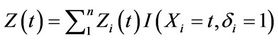, in words a continuous function equal to zero apart from at the observed failures in which it assumes the covariate value of the subject that fails. The number of observed failures k is given by If there are ties in the data our suggestion is to split them randomly although there are a number of other suggested ways of dealing with ties. All of the techniques described here require only superficial modification in order to accommodate any of these other approaches for dealing with ties.

1.3. Models

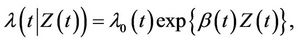
Insight is helped when we group the models together under as general a heading a possible. The most general model is then the non proportional hazards model written,

(1.1)

where is the conditional hazard function, the baseline hazard and the time-varying regression effect. Whenever has dimension greater than one we view as an inner product, having the same dimension as. In order to avoid problems of identifiability we assume that, if indeed time-dependent, has a clear interpretation such as the value of a prognostic factor measured over time, so that is precisely the regression effect of on the log hazard ratio at time t. The above model becomes a proportional hazards model under the restriction that a constant i.e. 

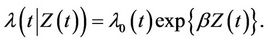(1.2)

O’Quigley and Stare [12] introduced the name “partially proportional hazards models” to describe models in which at least one component of the function is constrained to be constant. Such models can be shown to include the stratified proportional hazards model [13] whereby;

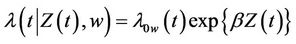(1.3)

as well as random effects models [12].

2. Model Based Probabilities

The probability structure of the model, needed in our development, is described in O’Quigley [1]. We recall the main results in this section. Most often time is viewed as a set of indices to certain stochastic processes, so that, for example, we consider to be a random variable having different distributions for different t. Also, the failure time variable T can be viewed as a non-negative random variable with distribution and, whenever the set of indices t to the stochastic process coincide with the support for T, then, not only can we talk about the random variables for which the distribution corresponds to 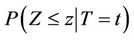but also marginal quantities such as the random variable having distribution. An important result concerning the conditional distribution of given follows. First we need the following:

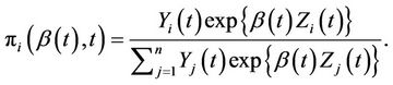
Definition 1. The discrete probabilities are given by;

(2.1)

Under (1.2), i.e. the constraint, the product of the’s over the observed failure times gives the partial likelihood [3]. When, is the empirical distribution that assigns equal weight to each sample subject in the risk set. Based upon the we have:

Definition 2. Moments of Z with respect to are given by;

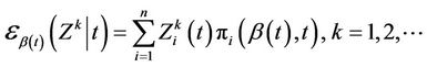(2.2)

Definition 3. In order to distinguish conditionally independent censoring from independent censoring we define where;

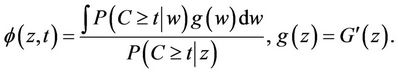
Note that when censoring does not depend upon z then will depend upon neither z or t and is, in fact, equal to one. Otherwise, under a conditionally independent censoring assumption, we can consistently estimate and we call this The following theorem underlies our development.

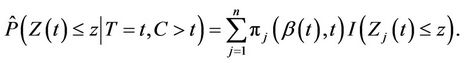
Theorem 1. Under model (1) and assuming known, the conditional distribution function of given is consistently estimated by  

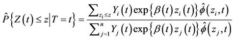(2.3)

Proof. (see [1])

Straightforward applications of Slutsky’s theorem enable us to claim the result continues to hold whenever is replaced by any consistent estimator, in particular the partial likelihood estimator when we assume the more restricted model (1.2). □

The theorem has many important consequences includeing;

Corollary 1. Under model (1) and an independent censorship, assuming known, the conditional distribution function of given is consistently estimated by

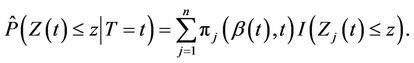(2.4)

Corollary 2. For a conditionally independent censoring mechanism we have 

(2.5)

Again simple applications of Slutsky’s theorem shows that the result still holds for replaced by any consistent estimate. When the hypothesis of proportionality of risks is correct then the result holds for the estimate. Having first defined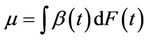, it is also of interest to consider the approximation;

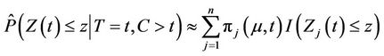(2.6)

and, for the case of an independent censoring mechanism,

(2.7)

For small samples it will be unrealistic to hope to obtain reliable estimates of for all of t so that, often, we take an estimate of some summary measure, in particular. It is in fact possible to estimate without estimating [11] although the usual partial likelyhood estimate does not accomplish this. In fact the partial likelihood estimate turns out to be equivalent to obtaining the solution of an estimating equation based upon and using as an estimate whereas, to consistently estimate, it is necessary to work with some consistent estimate of, in particular the Kaplan-Meier estimate. We firstly need some definition of what is being estimated when the data are generated by model (1.1) and we are working with model (1.2). This is contained in the following definition for.

Definition 4. Let be the constant value satisfying

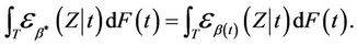(2.8)

The definition enables us to make sense out of using estimates based on (1.2) when the data are in fact generated by (1.1). Since we can view T as being random, whenever is not constant, we can think of having sampled from. The right hand side of the above equation is then a double expectation and the best fitting value under the constraint that We can show the existence and uniqueness of solutions to Equation (8) [11] More importantly, can be shown to have the following three properties; 1) under model (1.2); 2) under a subclass of the Harrington-Fleming models, and 3) for general situations Estimates of are discussed in [2,11] and, in the light of the foregoing, we can take these as estimates of. We also have the further two corollaries to Therorem 1:

Corollary 3. For, provides consistent estimates of, under model (1). In particular provides consistent estimates of, under model (1.2).

Furthermore, once again under the model, if we let thenCorollary 4. Under model (1.2), is consistently estimated by.

Theorem 1 and its corollaries provide the ingredients necessary to a construction from which several tests can be derived.

3. Important Empirical Processes

Consider the partial scores introduced by Wei [14];

(3.1)

Wei was interested in goodness of fit for the two group problem and based a test on, large values indicating departures away from proportional hazards in the direction of non proportional hazards. Considerable exploration of this idea, and substantial generalization via the use of martingale based residuals, has been carried out by Lin, Wei and Ying [15]. These investigations showed that we could work with a much broader class of statistics that those based on the score so that a wide choice of functions, potentially describing different kinds of departures from the model, are available. Apart from the two group case, limiting distributions are complicated and usually approximated via simulation. Although the driving idea is that of goodness of fit, the same techniques can be applied to testing for the presence of regression effects against a null hypothesis that Furthermore, working directly with the increments of the process rather than the process itself, we can derive related processes for which the limiting distributions are available analytically. From the previous section the increments of the process at have mean and variance. We can view these increments as being independent [16,17]. Thus only the existence of the variance is necessary in order to carry out appropriate standardization and to be able to appeal to the functional central limit theorem. We can then treat our observed process as though arising from a Brownian motion process. Simple calculations allow us to also work with the Brownian bridge, integrated Brownian motion and reflected Brownian motion, processes which will be useful under particular alternative to the model specified under the null hypothesis. Consider the process, , in which 

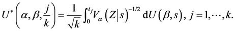(3.2)

where. This process is only defined on k equispaced points of the interval (0, 1] but we extend our definition to the whole interval via linear interpolation so that, for u in the interval to, we write;

As n goes to infinity, under the usual Breslow and Crowley conditions, then we have that, for each j (),converges in distribution to a Gaussian process with mean zero and variance equal to. This follows directly from Donsker’s theorem. Replacing by a consistent estimate leaves asymptotic properties unaltered.

3.1. Some Remarks on the Notation

Various aspects of the statistic will be used to construct different tests. We choose the * symbol to indicate some kind of standardization as opposed to the non standardized U. The variance and the number of failure points are used to carry out the standardization. Added flexibility in test construction can be achieved by using the two parameters, and, rather than a single parameter. In practice these are replaced by quantities which are either fixed or estimated under some hypothesis. For goodness of fit procedures which we consider later we will only use a single parameter, typically. Goodness of fit tests are most usefully viewed as tests of hypotheses of the form. A test then of a hypothesis may not seem very different. This is true in principle. However, for a test of, we need keep in mind not only behaviour under the null but also under the alternative. Because of this it is often advantageous, under a null hypothesis of, to work with and in the expression. Under the null, remains consistent for the value 0 and, in the light of Slutsky’s theorem, the large sample distribution of the test statistics will not be affected. Under the alternative however things look different. The increments of the process at no longer have mean and adding them up will indicate departures from the null. But the denominator is also affected and, in order to keep the variance estimate not only correct but also as small as we can, it is preferable to use the value rather than zero.

3.2. Some Properties of

A very wide range of possible tests can be based upon the statistic and we consider a number of these below. Well known tests such as the partial likelyhood score test obtain as a special cases. First we need to make some observations on the properties of under different values of, and u.

Lemma 1. The process, for all finite and is continuous on [0, 1]. Also

Lemma 2. Under model 1.2 converges in probability to zero.

Lemma 3. Suppose that, then

converges in probability to v.

Proofs of the above lemmas are all immediate. Since the increments of the process are asymptotically independent we can treat (as well as

under some hypothesized) as though it were Brownian motion. From Corollary 3 we have that provides consistent estimates of, under model (1.2) and that is consistent for.

Therefore, at, the variance of

goes to the value one, as a simple application of Slutsky’s theorem. A further application of Slutsky’s theorem, together with theorems of Cox and Andersen and Gill [16,17] provide that the increments are asymptotically uncorrelated. Let

Then

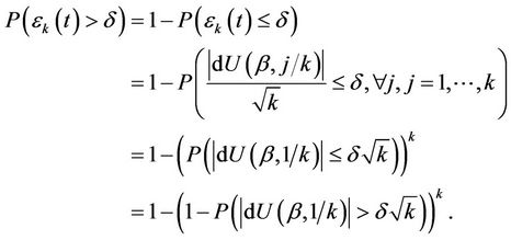
Applying the Chebyshev inequality,

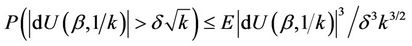
from which 

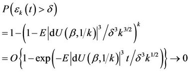
as k becomes large. Apart from the necessity for the existence of the third moment of Z we also require that, as k increases, the fluctuations of the process between successive failures become sufficiently small in probability, the so called tightness of the process [18]. We can assume this holds in real applications. We then conclude from Donsker’s theorem that converges in distribution to Brownian motion. Replacing by a consistent estimate leaves asymptotic properties unaltered. Suppose that the assumption of zero effect, i.e., is incorrect, and, in particular, that is a smoothly changing monotonic function of time. Without losing generality we will assume this monotonicity to be an increasing one. Now, at each time point t, instead of subtracting off from the observed value of Z at that point, we subtract instead. The variance is also impacted but the variance is always positive (thereby impacting the average size but not the average sign of the increments). So, we will observe a positive trend in the standardized residuals, the early ones tending to be too large and the later ones tending to be too large also but negatively. A good model for this, at least as a first approximation, would be Brownian motion with drift [1]. For our purposes we note that, moving away from the model of zero regression effects, we anticipate observing some trend rather than zero mean Brownian motion. For decreasing, the same argument holds leading to an approximation of Brownian motion with drift but with the sign changed. These assertions follow when is monotone. Now suppose that is not monotone. There are two cases of interest. The first is where is broadly monotone, by which we mean the following. Divide the time interval into non overlapping time segments and take the average value of for each segment. We then suppose that the average value of, over the different time segments, is monotone. We could make this intuitive idea more precise if needed. For this case we would expect, again, the procedure to work well. The second case of interest is where changes over the time period in question in a way that has no obvious pattern or trend. We would not expect to be able to detect such behavior and the power of the test procedures would be low. We would most likely conclude that there is no effect, a conclusion that, even though not correct, would be reasonable, at least as an approximation.

4. Nonand Partially Proportional Hazards Models

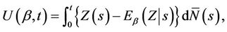
The Brownian motion approximations of the above section extend immediately to the case of non proportional hazards and partially proportional hazards models. The generalization of Equation (1) is natural and would lead to an unstandardized score; 

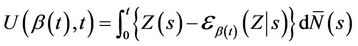(4.1)

and, as before, under the null hypothesis that is correctly specified the function will be a sum of zero mean random variables. The range of possible alternative hypotheses is large and, mostly, we will not wish to consider anything too complex. Often the alternative hypothesis will specify an ordering, or a non zero value, for just one of the components of a vector values. In the exact same way as in the previous section, all of the calculations lean upon the main theorem and its corollaries. The increments of the process

at t = X_i have mean and variance. A little bit of extra care is needed, in practice, in order to maintain the view of the independence of these increments. When is known there is no problem but if, as usually happens, we wish to use estimates, then, for asymptotic theory to still hold, we require the sample size (number of failures) to become infinite relative to the dimension of. Thus, if we wish to estimate the whole function, then some restrictions will be needed because, full generality implies an infinite dimensional parameter. For the stratified model and, generally, partially proportional hazards models, the problem does not arise because we do not estimate.

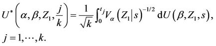
The sequentially standardized process will now be written, in which

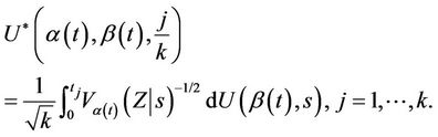
where. This process can be made to cover the whole interval (0, 1] continuously by interpolating in exactly the same way as in the previous section. For this process we reach the same conclusion, i.e., that as n goes to infinity, under the usual Breslow and Crowley conditions [17], then we have that, for each j (),converges in distribution to a Gaussian process with mean zero and variance equal to. The only potential difficulty is making use of Slutsky’s theorem whereby, if we replace and by consistent estimates the result still holds. The issue is that of having consistent estimates, which for an infinite dimensional unrestricted parameter we can not achieve. The solution is simply to either restrict these functions or to work with the stratified models in which we do not need to estimate them. Subsection 3.1 applies equally well here if we replace and by and. The lemmas of the above section describing the properties of apply equally we if we are working with, specifically, the process , for all finite and is continuous on [0, 1] and under model 1.2 converges in probability to zero and for, converges in probability to v. Since the increments of the process are asymptotically independent we will treat (as well as under some hypothesized) as though it were Brownian motion.

5. Test Statistics

Several tests of point hypotheses can be constructed based on the theory of the previous section. These tests can also be used to construct test based confidence intervals of parameter estimates, obtained as solutions to an estimating equation. Among these tests are the following.

5.1. Distance Travelled at Time t

At time t, under the null hypothesis that, often a hypothesis of absence of effect in which case, we have that can be approximated by a normal distribution with mean zero and variance t. A p-value corresponding to the null hypothesis is then obtained from

This p-value is for a one-sided test in the direction of the alternative For a one-sided alternative in the opposite direction we would use;

and, for a two sided alternative, we would, as usual, consider the absolute value of the test statistic and multiply by two. Under the alternative, say, if we take the first two terms of a Taylor series expansion of about, we can deduce that a good approximation for this would be Brownian motion with drift. At time t this is then a good test for absence of effect (Brownian motion) against a proportional hazards alternative (Brownian motion with drift), good in the sense that type I error is controlled for and, under these alternatives, the test has good power properties. Power will be maximized by using the whole time interval, i.e., taking Nonetheless there may be situations in which we may opt to take a value of t less than one. If we know for instance that, under both the null and the alternative we can exclude the possibility of effects being persistent beyond some time say, i.e., the hazard ratios beyond that point should be one or very close to that, then we will achieve greater power by taking t to be less than one, specifically some value around. A confidence interval for can be obtained using normal approximations or by constructing the interval such that for any point b contained in the interval a test of the null hypothesis, , is not rejected.

5.2. Greatest Distance from Origin at Time t

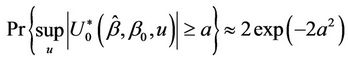
In cases where we wish to consider values of t less than one, we may have knowledge of some of interest. Otherwise we might want to consider several possible values of. Control on Type I error will be lost unless specific account is made of the multiplicity of tests. One simple way to address this issue is to consider the maximum value achieved by the process during the interval Again we can appeal to known results for some well known functions of Brownian motion. In particular we have;

Under the null and proportional hazards alternatives this test, as opposed to the usual score test, would lose power comparable to carrying out a two sided rather than a one-sided test. Under non-proportional hazards alternatives this test could be of use, an extreme example being crossing hazards where the usual score test may have power close to zero. As the absolute value of the hazard ratio increases so would the maximum distance from the origin.

5.3. Brownian Bridge Test

Since we are viewing the process as though it were a realization of a Brownian motion, we can consider some other well known functions of Brownian motion. Consider then the bridged process;

Definition 5. The bridged process is defined by the transformation

Lemma 4. The process converges in distribution to the Brownian bridge, in particular, for large samples, and

The Brownian bridge, also referred to as tied down Brownian motion for the obvious reason that at and the process takes the value 0, will not be particularly useful for carrying out a test at. It is more useful to consider, as a test statistic, the greatest distance of the bridged process from the time axis. We can then appeal to;

Lemma 5.

(5.1)

which follows as a large sample result since;

This is an alternating sign series and therefore, if we stop the series at k = 2 the error is bounded by which for most values of a that we will be interested in will be small enough to ignore. For alternatives to the null hypothesis () belonging to the proportional hazards class, the Brownian bridge test will be less powerful than the distance from origin test. It is more useful under alternatives of a non-proportional hazards nature, in particular an alternative in which is close to zero, a situation we might anticipate when the hazard functions cross over. Its main use, in our view, is in testing goodness of fit, i.e., a hypothesis test of the form [1].

5.4. Reflected Brownian Motion

An interesting property of Brownian motion is the following. Let be Brownian motion, choose some positive value r and define the process in the following way: If then If then. It is easily shown that the reflected process is also Brownian motion. Choosing r to be negative and defining accordingly we have the same result. The process coincides exactly with until such a time as a barrier is reached. We can imagine this barrier as a mirror and beyond the barrier the process is a simple reflection of. So, consider the process defined to be if and to be equal to if.

Lemma 6. The process converges in distribution to Brownian motion, in particular, for large samples, and

Under proportional hazards there is no obvious role to be played by U^r. However, imagine a non-proportional hazards alternative where the effect reverses at some point, the so-called crossing hazards problem. The statistic would increase up to some point and then decrease back to a value close to zero. If we knew this point, or had some reasons for guessing it in advance, thenwe could work with instead of . A judicious choice of the point of reflection would result in a test statistic that continues to increase under such an alternative so that a distance from the origin test might have reasonable power. In practice we may not have any ideas on a potential point of reflection. We could then consider trying a whole class of points of reflection and choosing that point which results in the greatest test statistic. A bound for a supremum type test can be derived by applying the results of Davies [19,20]. Under the alternative hypothesis we could imagine increments of the same sign being added together until the value r is reached, at which point the sign of the increments changes. Under the alternative hypothesis the absolute value of the increments is strictly greater than zero. Under the null, r is not defined and, following the usual standardization, this set up fits in with that of Davies [19, 20]. We can define to be the time point satisfying A two-sided test can then be based on the statistic Inference can then be based upon; 

(5.2)

where Ф denotes the cumulative normal distribution function, and where is the autocorrelation function between and. In general the autocorrelation function , needed to evaluate the test statistic is unknown. However, it can be consistently estimated using bootstrap resampling methods. For and taken as fixed, we can take bootstrap samples from which several pairs of and can be obtained. Using these pairs, an empirical, i.e. product moment, correlation coefficient can be calculated. Under the usual conditions [21,22], the empirical estimate provides a consistent estimate of the true value. This sampling strategy is investigated in related work by O’Quigley and Natarajan [23].

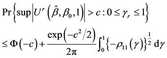
Davies also suggests an approximation in which the autocorrelation is not needed. This may be written down as

(5.3)

where the, ranging over (L, U), are the turning points of and M is the observed maximum of.

Turning points only occur at the k distinct failure times and, to keep the notation consistent with that of the next section, it suffices to take as being located half way between adjacent failures, and any value greater than the largest failure time. We would though require different inferential procedures for this.

5.5. Partial Likelihood Score Test

Suppose that we wish to test and instead of we choose to work with. In the light of Slutsky’s theorem it is readily seen that the large sample null distributions of the two test statistics are the same. Next, instead of standardizing by at each we take a simple average of such quantities, over the observed failures. To see this, note that is consistent for Rather than integrate with respect to it is more common, in the counting process context, to integrate with respect to, the two coinciding in the absence of censoring. It is also more common to fix in at its null value zero. This gives us:

Definition 6. The empirical average conditional variance, is defined as

.

If, in Equation (3.2), we replace by then the distance from origin test at time coincides exactly with the partial likelihood score test. Indeed this observation could be used to construct a characterization of the partial likelihood score test. In epidemiological applications it is often assumed that the conditional variance, is constant through time. Otherwise time independence is often a good approximation to the true situation and gives further motivation to the partial likelihood test.

6. Multivariate Model

In practice it is the multivariate setting that we are most interested in; testing for the existence of effects in the presence of related covariates, or possibly testing the combined effects of several covariates. In this work we give very little specific attention to the multivariate setting, not because we do not feel it to be important but because the univariate extensions are almost always rather obvious and the main concepts come through more clearly in the relatively notationally uncluttered univariate case. Nonetheless, some thought is on occasion required. The basic theorem giving a consistent estimate of the distribution of the covariate at each time point t applies equally well when the covariate is multidimensional. Everything follows through in the same way and there is no need for additional theorems. In the multivariate case the product becomes a vector or inner product, a simple linear sum of the components of and the corresponding components of Suppose, for simplicity, that is two dimensional so that Then the give our estimate for the joint distribution of at time t. As for any multi-dimensional distribution if we wish to consider only the marginal distribution of, say, then we simply sum the over the variable. In practice we work with the, defined to be of the highest dimension that we are interested in, for the problem in hand, and simply sum over the subsets of vector Z needed. To be completely concrete let us return to the partial scores, 

(6.1)

defined previously for the univariate case. Both and are vectors of the same dimension. So also is then. The vector is made up of the component marginal processes any of which we may be interested in. For each marginal covariate, let’s say for instance, we also calculate and we can do this either by first working out the marginal distribution of or just by summing over the joint probabilities. The result is the same and it is no doubt easier to work out all expectations with the respect to the joint distribution. Let us then write; 

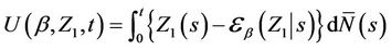(6.2)

where the subscript “1” denotes the first component of the vector. The interesting thing is that does not require any such additional notation, depending only on the joint. As for the univariate case we can work with any function of the random vector Z, the expectation of the function being readily estimated by an application of an immediate generalization of Corollary 3. Note that the process we are constructing is not the same one that we would obtain were we to simply work with only. This is because the involve a univariate Z in the former case and a multivariate Z in the latter. The increments of the process at have mean and variance. As before, these increments can be taken to be independent [16,17] so that only the existence of the variance is necessary to be able to appeal to the functional central limit theorem. This observed process will also be treated as though arising from a Brownian motion process. The same calculations as above allow us to also work with the Brownian bridge, integrated Brownian motion and reflected Brownian motion. Our development is entirely analogous to that for the univariate case and we consider now the process, in which 

where. This process is only defined on k equispaced points of the interval (0, 1] and, again, we extend our definition to the whole interval so that, for we can write as;

As n goes to infinity, under the usual Breslow and Crowley conditions [17], then we have that, for each j (),converges in distribution to a Gaussian process with mean zero and variance equal to. This follows in the same way as for the univariate case, directly from Donsker’s theorem. Replacing by a consistent estimate leaves asymptotic properties unaltered.

6.1. Some Further Remarks on the Notation

The notation is a little heavy but becomes even heavier if we wish to treat the situation in great generality. The first component of Z is but of course this could be any component. Indeed can itself be a vector, some collection of components of Z and, once we see the basic idea, it is clear what to do even though the notation starts to become slightly cumbersome. As for the notation, , in which there is only one Z and no need to specify it, the * symbol continues to indicate standardization by the variance and number of failure points. For the multivariate situation, the two parameters, and, are themselves, both vectors. The parameter which indexes the variance will be, in practice, the estimated full vector, i.e., Note that, as for the process we use, for the first argument to this function, the unrestricted estimate. Exactly the same applies here. In the numerator however, under some hypothesis for, say then, for the increments, we would have fixed at and the other components of the vector replaced by their restricted estimates, i.e., zeros of the estimating equations in which

6.2. Some Properties of

The same range of possible tests as before can be based upon the statistic. To support this it is worth noting:

Lemma 7. The process, for all finite and is continuous on [0, 1]. Also

Lemma 8. Under model 2 converges in probability to zero.

Lemma 9. Suppose that, then

converges in probability to.

Since the increments of the process are asymptotically independent we can treat (as well as under some hypothesized) as though it were Brownian motion.

6.3. Tests in the Multivariate Setting

When we carry out a test of it is important to keep in mind the alternative hypothesis which is, usually, together with unspecified. Such a test can be carried out using where, for the second argument, the component is replaced by and the other components by estimates with the constraint that is fixed at. Assuming our model is correct, or a good enough approximation, then we are testing for the effects of having “accounted for” the effects of the other covariates. The somewhat imprecise notion “having accounted for” is made precise in the context of a model. It is not of course the same test as that based on a model with only included as a covariate.

Another situation of interest in the multivariate setting is one where we wish to test simultaneously for more than one effect. This situation can come under one of two headings. The first, analogous to an analysis of variance, is where we wish to see if there exists any effect without being particularly concerned about which component or components of the vector Z may be causing the effect. As for an analysis of variance if we reject the global null we would probably wish to investigate further to determine which of the components appears to be the cause. The second is where we use, for the sake of argument, two covariates to represent a single entity, for instance 3 levels of treatment. Testing for whether or not treatment has an impact would require us to simultaneously consider the two covariates defining the groups. We would then consider, for a two variable model, is a vector with components and, step functions with discontinuities at the points, , where they take the values and respectively. For this two dimensional case we consider the increments in the process

at, having mean

and variance

The remaining steps now follow through just as in the one dimensional case, and being replaced by and respectively, and the conditional expectations, variances and covariances being replaced using analogous results to Corollaries 3 and 4.

7. An Example

The classical example studied in Cox’s famous 1972 paper [3] concerning the two sample problem in a clinical trial in leukemia has been re-examined by several authors and we reconsider those data in the light of the work here. Our development sidesteps the issue of ties, a problem of sufficient importance for the Freireich data that it warranted lengthy discussion in Cox’s paper. Here we simply used a random split, although all of the suggested approaches for dealing with ties (see for example Kalbfleisch and Prentice [13] are accommodated without any additional difficulty. The distance from the origin at the maximum follow up time was equal to 3.92 (p < 0.001), a result which is to be anticipated since the proportional hazards assumption is known to be a good one for these data, and effects are strong. The partial likelyhood test produced the figure 3.94, confirming, at least here, the agreement we would expect given that the estimated conditional variance of the covariate given time is fairly constant with time itself. If the process is reflected at the time point t = 12, roughly the marginal median, then we obtain the value 0.58 which is what we might well expect. On the other hand if we use the reflected process, maximized across all potential times, then we obtain, again, a p-value less than 0.001 suggesting that little has been sacrificed by this more general approach even when the proportional hazards assumption appears well founded.

REFERENCES

- J. O’Quigley, “Khmaladze-Type Graphical Evaluation of the Proportional Hazards Assumption,” Biometrika, Vol. 90, No. 3, 2003, pp. 577-584. doi:10.1093/biomet/90.3.577
- R. Xu and J. O’Quigley, “Proportional Hazards Estimate of the Conditional Survival Function,” Journal of the Royal Statistical Society: Series B, Vol. 62, No. 4, 2000, pp. 667-680. doi:10.1111/1467-9868.00256
- D. R. Cox, “Regression Models and Life Tables (with discussion),” Journal of the Royal Statistical Society: Series B, Vol. 34, 1972, pp. 187-220.
- T. Lancaster and S. Nickell, “The Analysis of Re-Employment Probabilities for the Unemployed,” Journal of the Royal Statistical Society, Series A, Vol. 143, No. 2, 1980, pp. 141-165. doi:10.2307/2981986
- M. H. Gail, S. Wieand and S. Piantadosi, “Biased Estimates of Treatment Effect in Randomized Experiments with Nonlinear Regressions and Omitted Covariates,” Biometrika, Vol. 71, No. 3, 1984, pp. 431-444. doi:10.1093/biomet/71.3.431
- J. Bretagnolle and C. Huber-Carol, “Effects of Omitting Covariates in Cox’s Model for Survival Data,” Scandinavian Journal of Statistics, Vol. 15, 1988, pp. 125-138.
- J. O’Quigley and F. Pessione, “Score Tests for Homogeneity of Regression Effect in the Proportional Hazards Model,” Biometrics, Vol. 45, 1989, pp. 135-144. doi:10.2307/2532040
- J. O’Quigley and F. Pessione, “The Problem of a Covariate-Time Qualitative Interaction in a Survival Study,” Biometrics, Vol. 47, 1991, pp. 101-115. doi:10.2307/2532499
- G. L. Anderson and T. R. Fleming, “Model Misspecification in Proportional Hazards Regression,” Biometrika, Vol. 82, No. 3, 1995, pp. 527-541.
- I. Ford, J. Norrie and S. Ahmadi, “Model Inconsistency, Illustrated by the Cox Proportional Hazards Model,” Statistics in Medicine, Vol. 14, No. 8, 1995, pp. 735-746. doi:10.1002/sim.4780140804
- R. Xu and J. O’Quigley, “Estimating Average Regression Effect under Non Proportional Hazards,” Biostatistics, Vol. 1, 2000, pp. 23-39. doi:10.1093/biostatistics/1.4.423
- J. O’Quigley and J. Stare, “Proportional Hazard Models with Frailties and Random Effects,” Statistics in Medicine, Vol. 21, 2003, pp. 3219-3233. doi:10.1002/sim.1259
- J. Kalbfleisch and R. L. Prentice, “The Statistical Analysis of Failure Time Data,” Wiley, New York, 1980.
- L. J. Wei, “Testing Goodness of Fit for Proportional Hazards Model with Censored Observations,” Journal of the American Statistical Association, Vol. 79, 1984, pp. 649-652.
- D. Y. Lin, L. J. Wei and Z. Ying, “Checking the Cox Model with Cumulative Sums of Martingale-Based Residuals,” Biometrika, Vol. 80, No. 3, 1993, pp. 557-572. doi:10.1093/biomet/80.3.557
- D. R. Cox, “Partial Likelihood,” Biometrika, Vol. 63, 1975, pp. 269-276. doi:10.1093/biomet/62.2.269
- P. K. Andersen and R. D. Gill, “Cox’s Regression Model for Counting Processes: A Large Sample Study,” Annals of Statistics, Vol. 10, No. 4, 1982, pp. 1100-1121. doi:10.1214/aos/1176345976
- P. Billingsley, “Convergence of Probability Measures,” Wiley, New York, 1968.
- R. B. Davies, “Hypothesis Testing When a Nuisance Parameter Is Present Only under the Alternative,” Biometrika, Vol. 64, No. 2, 1977, pp. 247-254. doi:10.2307/2335690
- R. B. Davies, “Hypothesis Testing When a Nuisance Parameter Is Present Only under the Alternative,” Biometrika, Vol. 74, 1987, pp. 33-43.
- B. Efron, “Censored Data and the Bootstrap,” Journal of the American Statistical Association, Vol. 76, No. 374, 1981, pp. 312-319.
- B. Efron, “Nonparametric Estimates of Standard Error: The Jacknife, the Bootstrap and Other Resampling Methods,” Biometrika, Vol. 68, 1981, pp. 589-599. doi:10.1093/biomet/68.3.589
- J. O’Quigley and L. Natarajan, “Erosion of Regression Effect in a Survival Study,” Biometrics, Vol. 60, No. 2, 2004, pp. 344-351. doi:10.1111/j.0006-341X.2004.00178.x