Open Journal of Fluid Dynamics
Vol.2 No.4A(2012), Article ID:26365,6 pages DOI:10.4236/ojfd.2012.24A041
Numerical Analysis of Horizontal-Axis Wind Turbine Characteristics in Yawed Conditions
Department of Mechanical Systems Engineering, University of the Ryukyus, Okinawa, Japan
Email: m-suzuki@tec.u-ryukyu.ac.jp
Received September 27, 2012; revised November 9, 2012; accepted November 18, 2012
Keywords: Wind Turbine; Yawed Flow; CFD; Unsteady Rotor Aerodynamics; Performance
ABSTRACT
Computational fluid dynamics (CFD) modeling and experiments have both advantages and disadvantages. Doing both can be complementary, and we can expect more effective understanding of the phenomenon. It is useful to utilize CFD as an efficient tool for the turbomachinery and can complement uncertain experimental results. However the CFD simulation takes a long time for a design in generally. It is need to reduce the calculation time for many design conditions. In this paper, it is attempted to obtain the more accurate characteristics of a wind turbine in yawed flow conditions for a short time, using a few grid points. It is discussed for the reliability of the experimental results and the CFD results.
1. Introduction
Computational fluid dynamics (CFD) modeling and experiments have both advantages and disadvantages. Doing both can be complementary, and we can expect more effective understanding of the phenomenon. Although CFD has more advantages than experiments for the prediction where experiments are difficult to carry out, generally when compared with experimental results, it is difficult to obtain reliable results for a large domain by using CFD. However, it is possible to obtain useful CFD results based on verification by the experimental results. Moreover, experiments cannot deliver correct results for any arbitrary condition due to limitations to experimental equipment, measurement errors and problems with measurement systems. It is useful to utilize CFD as an efficient tool for the turbomachinery and can complement uncertain experimental results. However the CFD simulation takes a long calculation time for a design in generally. It is need to reduce the calculation time for many design conditions. In this paper, it is attempted to solve the more accurate characteristics of a wind turbine for a short time even a personal computer, using coarse grid [1]. In this paper the wind turbine characteristics of the yawed condition are discussed including the reliability of the experimental results and the CFD results.
2. Numerical Method
The in-house code used is an incompressible finite volume Navier-Stokes solver which is developed originally. The solver is based on structured grids and the use of curve-linear boundary fitted coordinates. The grid arrangement is collocated (Perić et al. [2]) and the Rhie and Chow interpolation method [3] is used. The SIMPLE algorithm (Patankar [4]) is used for pressure-velocity coupling. The convection term is calculated using the QUICK scheme (Leonard [5]) and the other terms in space are calculated using the 2nd order difference schemes. It is well known that sophisticated turbulence models do not always produce better results than the very simple models. For practical applications that are computationally expensive it is often wiser to use a simple approach. Therefore the proven and computationally efficient Launder-Sharma low-Reynolds-number k-e turbulence model [6] is used in this report.
3. Wind Turbine and Aerodynamic Force Acting to Blade
Figure 1 shows a schematic view of experimental apparatus for a wind turbine carried out by Vermeer [7]. A two bladed wind turbine is situated in front of the wind turbine. The wind turbine has diameter of 1.2 m and the blades consist of NACA 0012 airfoil and the chord length of 0.08 m. The experiment is conducted at wind velocity of 5 m/s, and the measured data are the wind velocity, the number of rotation, the torque, and the thrust. Moreover, Haans et al. [8,9] measure with the same experiment equipment about the thrust according to a yawed wind (0˚, ±15˚, ±30˚, ±45˚) of 5.5 m/s in speed
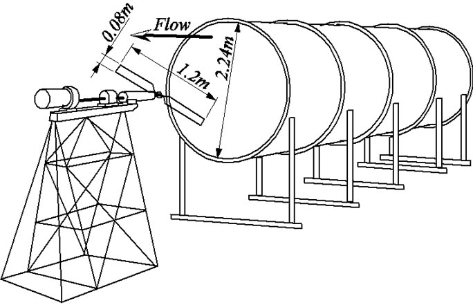
Figure 1. Schematic view of experimental apparatus of delft university of technology (Vermeer [7]).
and observe the tip vortex by flow visualization.
Figure 2 shows the relation with the fluid force acting to the blade element of the wind turbine with radius, r, the angle of pitch, q, the angle of attack, a, the lift, L, the drag, D, the tangential force, Ft, the axial force, Fa, i.e. thrust force, the axial velocity, Va, the tangential velocity, rw, the rotational speed, w, and the relative velocity, W.
Figure 3 shows the pitch angle, q, at each radius position, r. The pitch angle is changed linearly from qtip + 4˚ to qtip between nondimensional radius r/R = 0.3 and 0.9, and it is fixed to the pitch angle at tip between r/R = 0.9 and 1.0. The calculation is performed by a pitch angle at tip, that is, qtip = 2˚. Relation among the lift, L, the drag, D, the tangential force, Ft, and the axial force, Fa, in Figure 2 are written by:
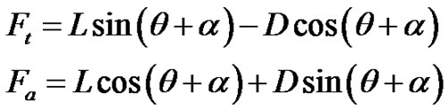 (1)
(1)
Under the no stall conditions which are small angle of attack, Equation (1) is approximated as follows:
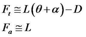 (2)
(2)
Since the axial force, Fa, i.e. thrust force, is predicted by the same accuracy as lift. On the other hand, since the tangential force, Ft, i.e., torque, is strongly influenced of drag, D, and it serves as the difference of the force by the lift and the drag, the produced force becomes small. For this reason, the predicted accuracy of torque is reduced than one of the thrust force.
Figure 4 shows the arrangement of yaw and azimuth angle.
The Reynolds number Re = UR/ν is expressed by the turbine radius, R, the wind velocity, U, and the kinematic viscosity of air, ν. The characteristics of wind turbine are expressed by the tip speed ratio, l, the power coefficient, CP, and the thrust coefficient, Ca,
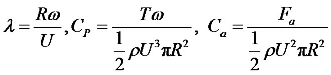 (3)
(3)
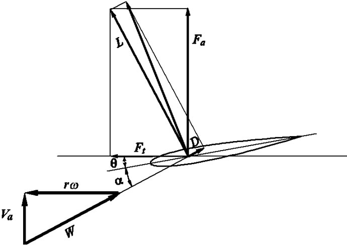
Figure 2. Fluid force acting a blade.
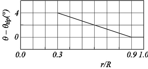
Figure 3. Pitch angle for radius of blade.
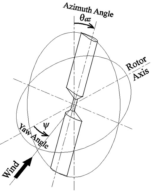
Figure 4. Arrangement of yaw and azimuth angle.
where the tip speed, Utip, the wind velocity, Va, the torque, T, the thrust, Fa, the air density, r.
4. Computational Grid
Figure 5 shows the upper half domain of the computational grid around the wind turbine rotor which is a sphere domain. The radius of the sphere is made into ten times of the rotor radius, and the external boundary is located at the 75 times of the chord length from the rotor axis. In addition, the internal diameter of the wind tunnel is about twice of wind turbine diameter, as shown in Figure 1, and the computational domain is sufficient wider than the experiment condition, that is 5 times of the internal diameter of a wind tunnel. The O-O type grid is enabling a suitable grid arrangement, being able to arrange many grid points along wing surface without
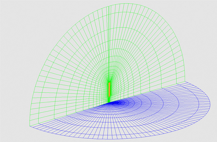
Figure 5. 3-D computational O-O grid around blade of wind turbine.
distributing many points to unnecessary parts. The number of grid points is 130 around the configuration, 56 points in the spanwise, 57 points normal to the surface direction, and the 414,960 points in total. The grid is generated using a algebraic grid generation method (Eriksson [10]) based on the transfinite interpolation method which gives 5 ´ 10−5 in a direction normal to the nearwall grid spacing to unit rotor radius, and y+ values of less than 0.65.
5. Comparison between Computation and Experiment in Non-Yawed Flow
Figure 6 shows the power coefficient of qtip = 2˚. The experimental results show the characteristics that the maximum power coefficient, CP appears at l = 7.5, the stall region appears below l = 6, and the power coefficient decreases from above l = 7.5, because the angle of attack becomes smaller as increase of tip speed ratio. The power coefficients are in good agreement with experimental results. The big difference between the computational and the experimental results produces near just after stall angle where the tip speed ratio is l = 6 ~ 3 [1]. Since the present turbulence models cannot fully predict the transition from laminar to turbulent flow, and cause to delay stall. About this, we will expect for development of a future turbulence model. Since the leading edge separation is completely occurred in the region less than l = 3 in tip speed ratio, it is comparatively easy to catch also in the CFD, and the results become nearly equal to ones of the experiment. For the region is larger than l = 6.75 in tip speed ratio which becomes small angle of attack not to stall, the characteristics can fully be predicted by the numerical computation.
Figure 7 shows the thrust coefficient. The computational results of a thrust coefficient, Ca agree well with the experimental results all over the region, because the thrust is dominated by the lift and little influence of a drag. Furthermore, the lift coefficient can expect accurate
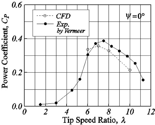
Figure 6. Power coefficients of non-yawed condition.
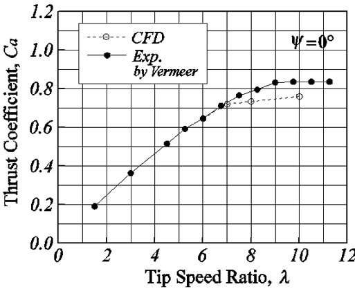
Figure 7. Thrust coefficients of non-yawed condition.
prediction for the CFD, because even the potential calculation is as small different as about 10% from the experimental result.
The thrust force is nearly equal to the lift, while the tangential force is strongly influenced of a drag, because it becomes the difference of L (a + q) and D from Equation (2), it turns into the small force of less than 10% as compared with a thrust force. For this reason, it is easy not only in numerical computation but also in the experiment to produce a big error for the tangential force.
6. Wind Turbine Characteristics in Yawed Flow
Haans et al. [8] measure only the thrust coefficient as experimental data, and the measurement about the power coefficient has not gone. For this reason, only thrust coefficients are compared with experimental results here. And assuming that only the turbine axis component of wind velocity influences the characteristics of the yawed flow, the simple wind turbine characteristics computed using the experimental data of ψ = 0˚ are also described together, that is, as characteristics of yawed flow:
 (4)
(4)
are introduced as the estimation equation, where CP(l, 0) and Ca(l, 0) are the power coefficient and thrust coefficient for the tip speed ratio at yaw angle of 0˚, respectively. In relation to this, Maeda et al. [11] have reported that the maximum power coefficients becomes in the non-yawed value times between cos2ψ and cos3ψ by the experiment.
Figures 8-10 show the thrust coefficients for ψ = ±15˚, ±30˚ and ±45˚. First, the computational fluid dynamics (CFD) results are compared with the simple prediction results (Cal.) calculated by Equation (4) using the experimental data of yawed angle ψ = 0˚ by Vermeer [6]. The results of Equation (4) are well in agreement with CFD results for ψ = 15˚, 30˚ and 45˚. For tip speed ratio, l = 8 and 10, although the difference in about ten percent has appeared, it is because the CFD results have the difference from the experiment data in the yawed angle 0˚. Thus, the result of the simple presumed formula and
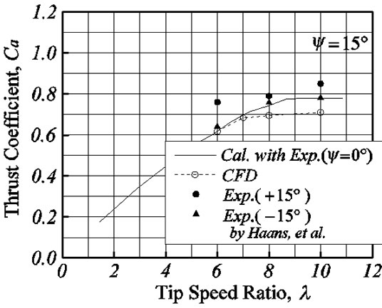
Figure 8. Thrust coefficients of 15˚ yawed angle.
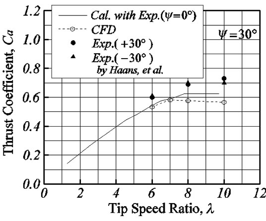
Figure 9. Thrust coefficients of 30˚ yawed angle.
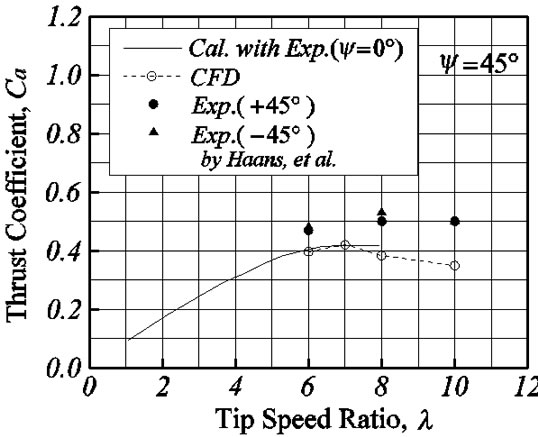
Figure 10. Thrust coefficients of 45˚ yawed angle.
CFD corresponds well, it is suggested that the cross flow along a surface of revolution does not influence to the thrust.
On the other hand, although the experimental results of ψ = 15˚ are well in agreement with a simple formula and the CFD, the experimental results become bigger value than the value predicted by CFD as large yaw angle such as ψ = 30˚ and 45˚. But the big error is also included in the experimental results of ψ = 15˚ shown in Figure 5. Essentially, since the flow becomes symmetrical for the positive/negative of yaw angle, the thrust coefficient must be in agreement. However the difference between positive and negative yaw angle appears 10% - 20% in the experimental results. Haans et al. [8] shows judgment because the velocity distribution of the wind tunnel exit does not become uniform. Thus, the uncertain element is also contained in the experimental result and we want to consider as the future work about the difference between the experiment and the CFD result.
Figures 11-13 show the power coefficient for the yaw angles ψ = 15˚, 30˚ and 45˚. The CFD results are compared with the simple prediction results (Cal.) calculated by Equation (4) using the experimental data of yaw angle ψ = 0˚. Although the CFD results of ψ = 0˚ is smaller, about 0.1, than the experimental result of power coefficient, the tendency is well in agreement for the tip speed ratio. About the yaw angle, ψ = 15˚, 30˚, 45˚, the results of a simple formula (4) and the results of CFD show good coincidence, and it is shown that the macroscopic amount of time averages like the thrust coefficient and the power coefficient can express the characteristic by the comparatively easy relation.
7. Fluctuation of Thrust and Power Coefficient Depending on Azimuth Angle
As described by the previous section, although it is thought that the time average power and thrust are predicted comparatively well in the simple formula (4), which is calculated using the characteristic of the nonyaw angle, in order to predict the fatigue load inflicted to wings, it is important to presume correctly the unsteady characteristic for the azimuth angle.
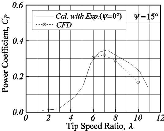
Figure 11. Power coefficients of 15˚ yaw angle.
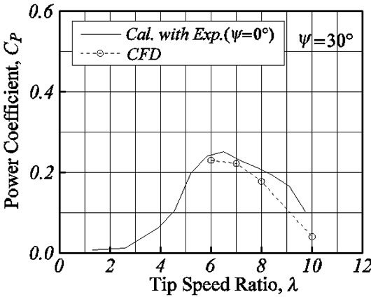
Figure 12. Power coefficients of 30˚ yaw angle.
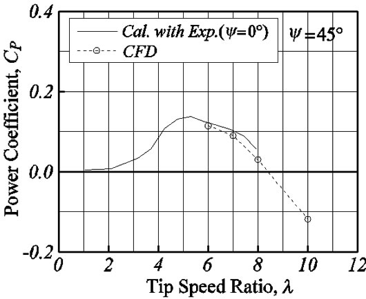
Figure 13. Power coefficients of 45˚ yaw angle.
Figures 14-16 show the fluctuation of thrust force, Ca, for azimuth angle, θaz. The range of thrust fluctuation for the azimuth angle increases in connection with the increase in the yaw angle, ψ, or the tip speed ratio, l, and the range of fluctuation has reached about 30% of the average value at l = 10 and ψ = 45˚. The thrust force is the maximum at θaz = 90˚ and the minimum at θaz = 250˚ for the tip speed ratio, l = 6, the maximum at θaz = 110˚ and the minimum at θaz = 30˚ for l = 8, and the maximum at θaz = 180˚ and the minimum at θaz = 0˚ for l = 10. The thrust force is smoothed by the two blades to be canceled with each other blade.
Figures 17-19 show the fluctuation of power for the azimuth angle. The amplitude of the power fluctuation also increases in connection with the increase in the yaw angle or the tip speed ratio, the range of fluctuation has reached the twice of average value for the yaw angle of ψ = 45˚. The power is the maximum at θaz = 140˚ and the minimum at θaz = 0˚ for l = 6, the maximum at θaz = 170˚ and the minimum at θaz = 5˚ for l = 8, and the maximum at θaz = 160˚ and the minimum at θaz = 350˚ for l = 10. The power of rotor is smoothed by the two blades to be canceled with each other blade. These show that the phase of the fluctuated waveform of the thrust force and the power tends to delay with the tip speed ratio.
8. Conclusions
While the CFD and the simple presumed formula are performed to grasp detailedly the wind turbine characteristics complementing the experimental results, the verification is performed by carrying out comparison and examination each other. The knowledge about the wind turbine characteristics of the yaw flow obtained by this study are shown as follows:
1) The simple calculation formula was introduced to presume the characteristics of the yaw flow.
2) The characteristics of the yaw flow are computed by the CFD, of which results are compared with the experimental results or the proposed simple calculation. It is
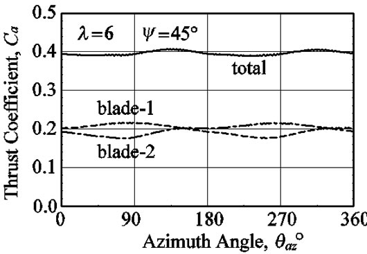
Figure 14. Fluctuation of thrust coefficients where the tip speed ratio is 6 and the yaw angle is 45˚.
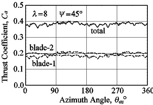
Figure 15. Fluctuation of thrust coefficients where the tip speed ratio is 8 and the yaw angle is 45˚.
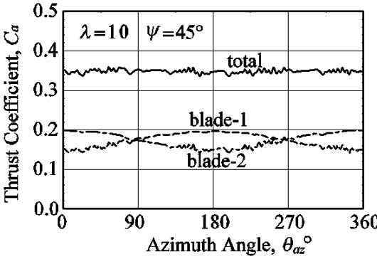
Figure 16. Fluctuation of thrust coefficients where the tip speed ratio is 10 and the yaw angle is 45˚.
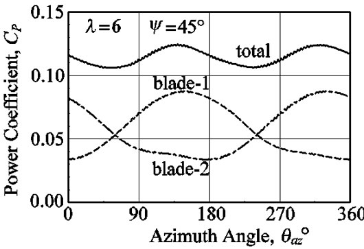
Figure 17. Fluctuation of power coefficients where the tip speed ratio is 6 and the yaw angle is 45˚.
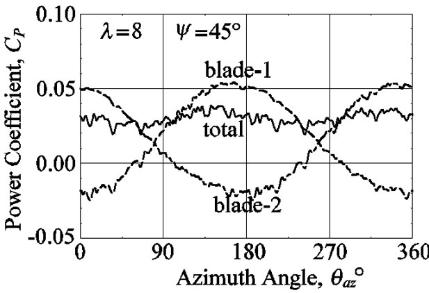
Figure 18. Fluctuation of power coefficients where the tip speed ratio is 8 and the yaw angle is 45˚.
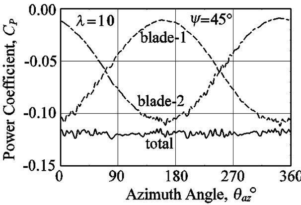
Figure 19. Fluctuation of power coefficients where the tip speed ratio is 10 and the yaw angle is 45˚.
expected that the influence of yawed flow can be estimated roughly by the simple presumed formula, because the results of the simple presumed formula are in agreement with the CFD. However, since the CFD and the simple estimation are in the tendency to appear smaller about 10% - 20% than the experimental results of thrust coefficient, the validation of accuracy including also experiment will be required after this. Moreover, the power coefficients show also the similar tendency between the simple formula and the CFD results.
3) The fluctuating torque and thrust force in one revolution affect the fatigue load of the blades. Although the total values of two blades are made smooth and the fluctuation decreases, the fluctuation of one blade is large. For example, in the yaw angle 45˚ and the tip speed ratio 10, the fluctuation ranges of the thrust coefficient and the torque coefficient reaches 3 times and twice of average value, respectively. Moreover, the tendency that the azimuth angle for which the thrust and the torque coefficient become the maximum and the minimum are delayed with the increase in the tip speed ratio appears.
REFERENCES
- M. Suzuki, “Evaluation of Experimental Results for Wind Turbine Characteristics by CFD,” Proceedings of the 9th International Symposium on Experimental and Computational Aero-thermodynamics of Internal Flows (ISAIF9), Gyeongju, 2009, Paper No. 1D-2.
- M. Perić, R. Kessier and G. Scheuerer, “Comparison of Finite-Volume Numerical Methods with Staggered and Collocated Grids,” Computers & Fluids, Vol. 16, No. 4, 1988, pp. 389-403. doi:10.1016/0045-7930(88)90024-2
- C. M. Rhie and W. L. Chow, “Numerical Study of the Turbulent Flow Past an Airfoil with Trailing Edge Separation,” AIAA Journal, Vol. 21, No. 11, 1983, pp. 1525- 1532. doi:10.2514/3.8284
- S. V. Patankar, “Numerical Heat Transfer and Fluid Flow,” McGraw-Hill, New York, 1980.
- B. P. Leonard, “A Stable and Accurate Convective Modeling Procedure Based on Quadratic Upstream Interpolation,” Computer Methods in Applied Mechanics and Engineering, Vol. 19, No. 1, 1979, pp. 59-98. doi:10.1016/0045-7825(79)90034-3
- B. E. Launder and B. I. Sharma, “Application of the Energy-Dissipation Model of Turbulence to the Calculation of Flow near a Spinning Disk,” Letters in Heat Mass Transfer, Vol. 1, 1974, pp. 131-138. doi:10.1016/0094-4548(74)90150-7
- N. J. Vermeer, “Performance measurements on a Rotor Model with Mie-Vanes in the Delft Open Jet Tunnel,” Institute for Wind Energy, Delft University of Technology, Delft, 1991, IW-91048R.
- W. Haans, T. Sant, G. van Kuik and G. van Bussel, “Measurement of Tip Vortex Paths in the Wake of a HAWT Under Yawed Flow Conditions,” Journal of Solar Energy Engineering, Vol. 127, No. 4, 2005, pp. 456-463. doi:10.1115/1.2037092
- W. Haans, T. Sant, G. van Kuik and G. van Bussel, “Stall in Yawed Flow Conditions: A Correlation of Blade Element Momentum Predictions with Experiments,” Journal of Solar Energy Engineering, Vol. 128, No. 4, 2006, pp. 472-480. doi:10.1115/1.2349545
- L. E. Eriksson, “Generation of Boundary Conforming Grids around Wing-Body Configurations Using Transfinite Interpolations,” AIAA Journal, Vol. 20, No. 10, 1982, pp. 1313-1320. doi:10.2514/3.7980
- T. Maeda, Y. Kamada, J. Suzuki and H. Fujioka, “Rotor Blade Sectional Performance under Yawed Inflow Conditions,” Journal of Solar Energy Engineering, Vol. 130, No. 3, 2008, Article ID: 031018. doi:10.1115/1.2931514