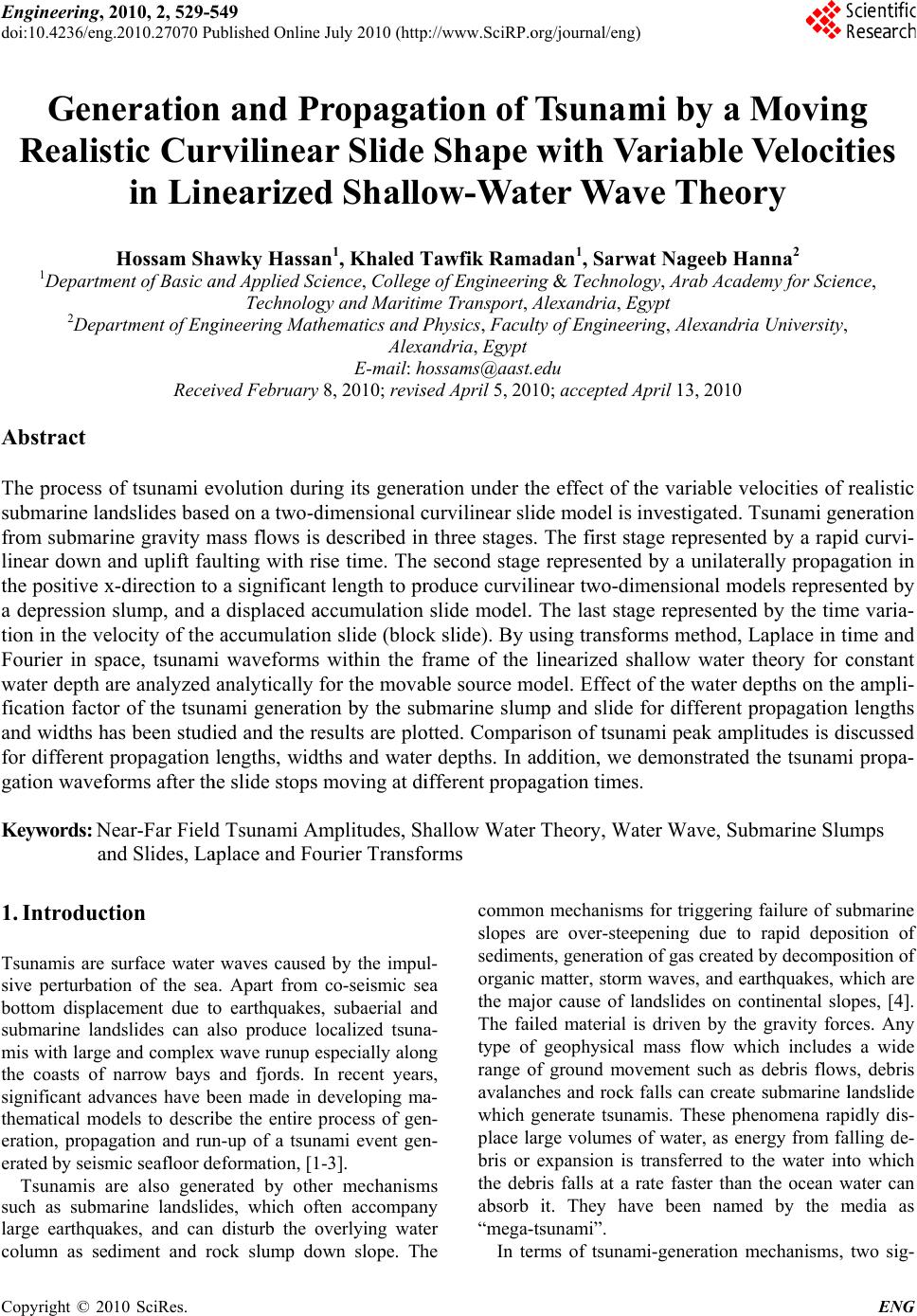Engineering,
doi:10.4236/en
g
Copyright © 2
0
Ge
n
Reali
s
1
Depart
m
2
Dep
a
Abstract
The process
submarine l
a
from subma
r
linear down
the positive
x
a depression
tion in the v
e
Fourier in s
p
water depth
a
fication fact
o
and widths
h
for different
gation wave
f
Keywords:
N
a
1. Introdu
c
Tsunamis are
sive perturba
t
b
ottom displ
a
submarine la
n
mis with larg
e
the coasts o
f
significant ad
v
thematical m
o
eration, prop
a
erated by seis
m
Tsunamis
a
such as sub
m
large earthqu
a
column as s
e
2010, 2, 529-
5
g
.2010.27070 P
u
0
10 SciRes.
n
eratio
n
s
tic Cu
r
in Li
n
Hossam S
h
m
ent of Basic
a
a
rtment of En
g
Rece
i
of tsunami
e
a
ndslides bas
e
r
ine gravity
m
and uplift fa
u
x
-direction t
o
slump, and
a
e
locity of th
e
p
ace, tsuna
m
a
re analyzed
o
r of the tsu
n
h
as been stud
propagation
f
orms after t
h
N
ea
r
-Far Fiel
d
a
nd Slides, L
a
c
tion
surface wate
r
t
ion of the se
a
a
cement due
t
n
dslides can
a
e
and comple
x
f
narrow bays
v
ances have
b
o
dels to descr
i
a
gation and ru
n
m
ic seafloor
d
a
re also gen
e
m
arine landsli
d
a
kes, and ca
n
e
diment and r
5
49
u
blished Onlin
e
n
and P
r
viline
a
n
earize
d
h
awky Hass
a
a
nd Applied S
c
Technolo
g
g
ineering Mat
h
i
ved
F
ebruary
e
volution dur
i
e
d on a two-
d
m
ass flows i
s
u
lting with r
i
o
a significa
n
a
displaced
a
e
accumulati
o
m
i waveform
s
analytically
n
ami generat
i
ied and the r
e
lengths, wid
h
e slide stops
d
Tsunami A
a
place and F
o
r
waves cause
d
a
. Apart from
t
o earthquake
s
a
lso produce
l
x
wave runup
e
and fjords.
I
b
een made in
d
i
be the entire
p
n
-up of a tsu
n
d
eformation, [
1
e
rated by oth
d
es, which o
f
n
disturb the
o
ock slump d
o
e
July 2010 (htt
p
ro p ag
a
a
r Slide
d
Shall
o
a
n
1
, Khaled
T
c
ience, Colleg
e
g
y and Mariti
m
h
ematics and
P
A
lex
a
8, 2010; revi
s
i
ng its gener
a
d
imensional
c
s
described i
n
i
se time. Th
e
n
t length to p
r
a
ccumulation
o
n slide (blo
c
s
within the
f
for the mov
a
i
on by the s
u
e
sults are pl
o
ths and wate
r
moving at d
i
m
plitudes, S
h
o
urier Transf
o
d
by the imp
u
co-seismic s
e
s
, subaerial a
n
l
ocalized tsun
a
e
specially alo
n
I
n recent yea
r
d
eveloping
m
a
p
rocess of ge
n
n
ami event ge
n
1
-3].
er mechanis
m
f
ten accompa
n
o
verlying wat
e
o
wn slope. T
h
p
://www.SciRP.
o
a
tion of
Shape
o
w-Wa
t
T
awfik Ra
m
e
of Engineeri
n
m
e Transpor
t
,
P
hysics,
F
acu
l
a
ndria, Egypt
h
.
s
ed April 5, 20
a
tion under t
h
c
urvilinear sl
i
n
three stage
s
e
second stag
r
oduce curvi
l
slide model
.
c
k slide). By
u
f
rame of the
a
ble source
m
u
bmarine slu
m
o
tted. Compa
r
r depths. In
a
i
fferent prop
a
h
allow Wate
r
o
rms
u
l-
e
a
n
d
a
-
n
g
r
s,
a
-
n
-
n
-
m
s
n
y
e
r
h
e
comm
o
slopes
sedim
e
organi
c
the ma
j
The fa
i
type o
f
range
o
avalan
c
which
p
lace l
a
b
ris or
the de
b
absorb
“mega
-
In t
e
o
rg/journal
/
eng
)
Tsuna
m
with
V
t
er Wa
v
m
adan
1
, Sar
w
n
g & Technol
o
Alexandria,
E
l
ty of Enginee
r
.
edu
10; accepted
A
h
e effect of
t
i
de model is
s
. The first st
e represente
d
l
inear two-di
m
.
The last sta
g
u
sing transfo
linearized s
h
m
odel. Effect
m
p and slide
r
ison of tsun
a
a
ddition, we
a
gation time
s
r
Theory, W
a
o
n mechanism
are ove
r
-ste
e
e
nts, generatio
n
c
matter, stor
m
j
or cause of l
a
i
led material
i
f
geophysical
o
f ground mo
v
c
hes and rock
generate tsun
a
a
rge volumes
expansion is
b
ris falls at a
r
it. They ha
v
-
tsunami”.
e
rms of tsuna
m
)
m
i by a
V
ariable
v
e The
o
w
at Nageeb
H
o
gy,
A
rab Aca
d
Eg
yp
t
r
ing,
A
lexand
r
A
pril 13, 2010
t
he variable
v
investigated.
a
ge represen
t
d
by a unilat
e
m
ensional m
o
g
e represent
e
rms method,
h
allow wate
r
of the water
d
for different
a
mi peak am
p
demonstrate
d
s
.
a
ter Wave, S
u
s for triggerin
e
pening due t
o
n
of gas creat
e
m
waves, and
e
a
ndslides on
c
i
s driven by t
h
mass flow
w
v
ement such
a
falls can crea
t
a
mis. These p
h
of water, as e
n
transferred t
o
r
ate faster tha
n
v
e been na
m
m
i-generation
Movin
Veloci
t
o
ry
H
anna
2
d
emy for Scie
n
r
ia University,
v
elocities of
r
Tsunami ge
n
t
ed by a rapi
d
e
rally propa
g
o
dels repres
e
e
d by the ti
m
Laplace in t
i
r
theory for
c
d
epths on th
e
propagation
p
litudes is d
i
d
the tsunam
i
u
bmarine Sl
u
g failure of s
u
o
rapid depo
s
e
d by decomp
o
e
arthquakes,
w
c
ontinental sl
o
h
e gravity for
c
w
hich include
s
a
s debris flow
t
e submarine
l
h
enomena rap
n
ergy from fa
o
the water in
t
n
the ocean
w
m
ed by the
m
mechanisms,
ENG
205
g
t
ies
n
ce,
r
ealistic
n
eration
d
curvi-
g
ation in
e
nted by
m
e varia-
i
me and
c
onstant
e
ampli-
lengths
i
scussed
i
propa-
u
mps
u
bmarine
s
ition of
o
sition of
w
hich are
o
pes, [4].
c
es. Any
s
a wide
s, debris
l
andslide
idly dis-
lling de-
t
o which
w
ater can
m
edia as
two sig-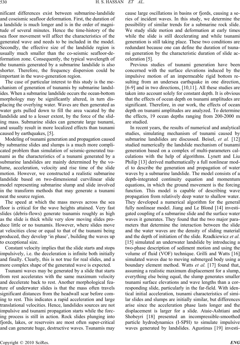

H. S. HASSAN ET AL. 530
nificant differences exist between submarine-landslide
and coseismic seafloor deformation. First, the duration of
a landslide is much longer and is in the order of magni-
tude of several minutes. Hence the time-history of the
sea floor movement will affect the characteristics of the
generated wave and needs to be included in the model.
Secondly, the effective size of the landslide region is
usually much smaller than the co-seismic seafloor-de-
formation zone. Consequently, the typical wavelength of
the tsunamis generated by a submarine landslide is also
shorter. Therefore, the frequency dispersion could be
important in the wave-generation region.
The case of particular interest to this study is the me-
chanism of generation of tsunamis by submarine landsl-
ides. When a submarine landslide occurs the ocean-bottom
morphology may be significantly altered, in turn dis-
placing the overlying water. Waves are then generated as
water gets pulled down to fill the area vacated by the
landslide and to a lesser extent, by the force of the slid-
ing mass. Submarine slides can generate large tsunami,
and usually result in more localized effects than tsunami
caused by earthquakes, [5].
Modeling of tsunami generation and propagation caused
by submarine slides and slumps is a much more compli-
cated problem than simulation of seismic-generated tsu-
nami as the characteristics of a tsunami generated by a
submarine landslides are mainly determined by the vo-
lume, acceleration, velocity and rise time of the slide
motion. However, we constructed a realistic submarine
landslide based on two-dimensional curvilinear slide
model representing submarine slump and slide involved
in the transform methods that may generate a tsunami
neat the source region.
The speed at which the mass moves across the sea
floor is critical for the wave heights attained. Very fast
slides (debris-flows) generate tsunamis roughly as high
as the slide is thick while very slow moving slides pro-
duce little or no tsunamis. However, where slides move
at velocities close or equal to that of the tsunami being
produced, they develop ‘in phase’, building the waves up
to exceptional size.
Constant velocity implies that the slide starts and stops
impulsively, i.e. the deceleration is infinite both initially
and finally. Clearly, this is not true for real slides, and a
more complex shape of the generated wave is expected.
Tsunami waves may be generated by a slide that starts
from rest accelerates with the same maximum velocity
and decelerate back to rest. Another morphological fea-
ture of underwater slides is that the mass often travels
significant distances from the headwall scar before com-
ing to rest. This indicates a rapid acceleration and large
translational velocities. Hence, landslides sources are not
impulsive and tsunami propagation starts while the forc-
ing process is still in action. Rock slides plunging into
fjords, lakes, or reservoirs are most often super-critical
and can generate huge, destructive waves. Tsunamis may
cause large oscillations in basins or fjords, causing a se-
ries of incident waves. In this study, we determine the
possibility of similar trends for a submarine rock slide.
We study slide motion and deformation at early times
while the slide is still decelerating and while tsunami
generation is still taking place. These two conditions are
redundant because one can define the duration of tsuna-
mi generation by the characteristic duration of slide ac-
celeration [5].
Previous studies of tsunami generation have been
concerned with the surface elevations induced by the
impulsive motion of an impermeable rigid bottom re-
sulting from an undersea earthquake in one direction,
[6-9] and in two directions, [10,11]. All these studies are
taken into account solely for constant depth. It is obvious
that the effects of ocean depth on tsunami amplitudes are
significant. Therefore, in our work, the effects of ocean
depth on tsunami amplitudes are analyzed. To determine
the effects, 19 ocean depths ranging from 200-2000 m
are studied.
In recent years, the results of numerical and analytical
studies, simulating mechanism of tsunami caused by
submarine landslides are discussed. Beisel, et al. [12]
studied numerically the landslide mechanism of tsunami
generation based on a complex of multi-parameters cal-
culations with the help of algorithms. Lynett and Liu
Philip [13] derived mathematically a full nonlinear mod-
el to describe the generation and propagation of water
waves by a submarine landslide. The model consists of a
depth-integrated continuity equation and momentum
equations, in which the ground movement is the forcing
function. This model is capable of describing wave
propagation from relatively deep water to shallow water.
They developed a numerical algorithm for the general
fully nonlinear model. Jiang and Le Blond [14] investi-
gated coupling of a submarine slide and the surface water
waves it generates. They found that the two major para-
meters that determine the interaction between the slide
and the water waves are the density of sliding material
and the depth of initiation of the slide. Rzadkiewicz et al.
[15] simulated an underwater landslide by introducing a
two-phase description of sediment motion and using the
volume of fluid (VOF) technique. Grilli and Watts [16]
simulated waves due to moving submerged body using a
boundary element method. Watts et al. [17] found that,
assuming a realistic maximum displacement for a slump,
everything else being equal, the slump generates smaller
tsunami surface elevations and wave lengths than a cor-
responding slide, particularly in the far-field. With iden-
tical initial acceleration, tsunami characteristics of simi-
lar slides and slumps are initially similar, but differences
arise since the acceleration phase lasts longer and the
displacement is larger for a slide. Ataie-Ashtiani and
Shobeyri [18] presented an incompressible-smoothed
particle hydrodynamics (I-SPH) to simulate impulsive
waves generated by landslides. Agustinus [19] investi-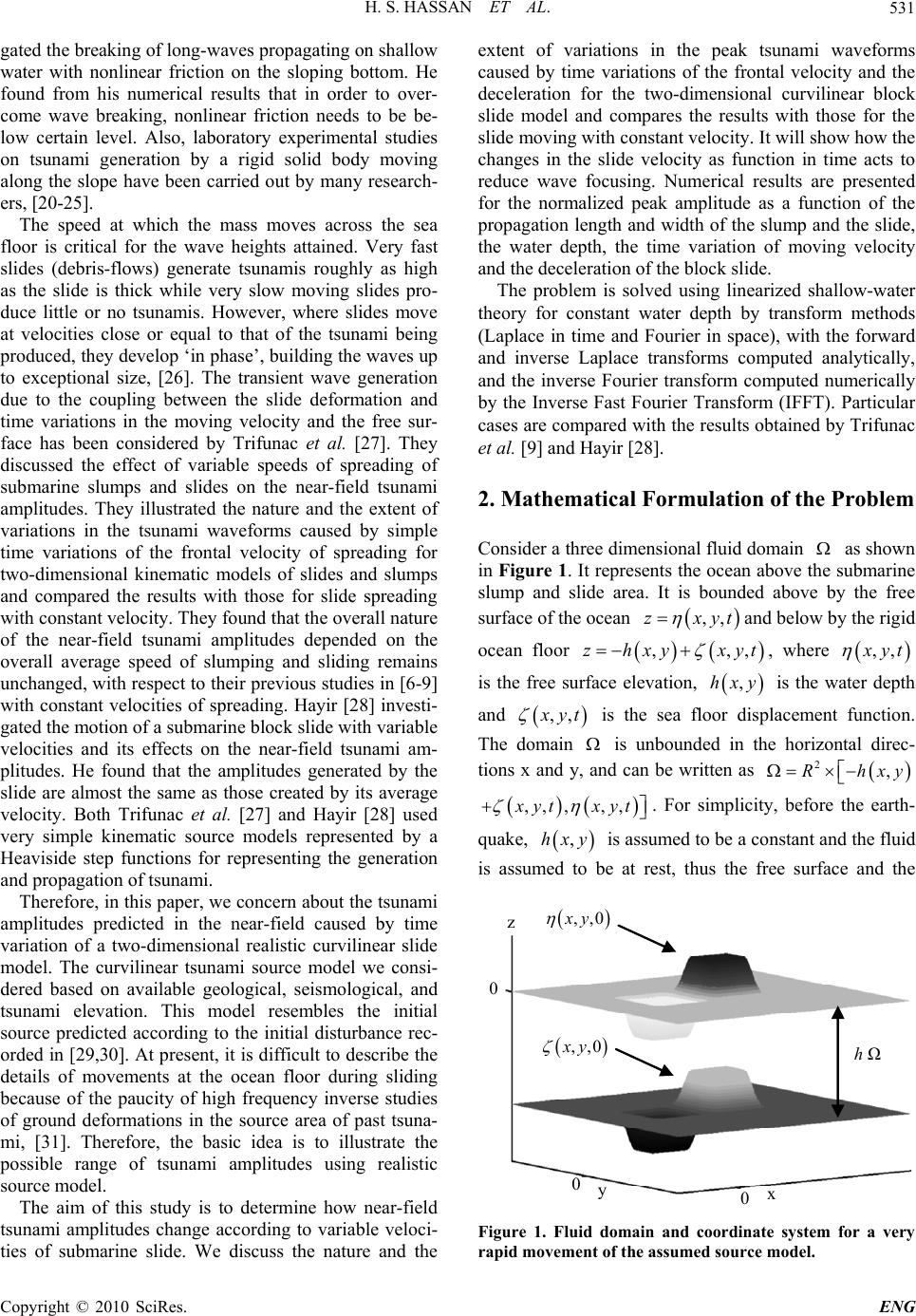

H. S. HASSAN ET AL. 531
gated the breaking of long-waves propagating on shallow
water with nonlinear friction on the sloping bottom. He
found from his numerical results that in order to over-
come wave breaking, nonlinear friction needs to be be-
low certain level. Also, laboratory experimental studies
on tsunami generation by a rigid solid body moving
along the slope have been carried out by many research-
ers, [20-25].
The speed at which the mass moves across the sea
floor is critical for the wave heights attained. Very fast
slides (debris-flows) generate tsunamis roughly as high
as the slide is thick while very slow moving slides pro-
duce little or no tsunamis. However, where slides move
at velocities close or equal to that of the tsunami being
produced, they develop ‘in phase’, building the waves up
to exceptional size, [26]. The transient wave generation
due to the coupling between the slide deformation and
time variations in the moving velocity and the free sur-
face has been considered by Trifunac et al. [27]. They
discussed the effect of variable speeds of spreading of
submarine slumps and slides on the near-field tsunami
amplitudes. They illustrated the nature and the extent of
variations in the tsunami waveforms caused by simple
time variations of the frontal velocity of spreading for
two-dimensional kinematic models of slides and slumps
and compared the results with those for slide spreading
with constant velocity. They found that the overall nature
of the near-field tsunami amplitudes depended on the
overall average speed of slumping and sliding remains
unchanged, with respect to their previous studies in [6-9]
with constant velocities of spreading. Hayir [28] investi-
gated the motion of a submarine block slide with variable
velocities and its effects on the near-field tsunami am-
plitudes. He found that the amplitudes generated by the
slide are almost the same as those created by its average
velocity. Both Trifunac et al. [27] and Hayir [28] used
very simple kinematic source models represented by a
Heaviside step functions for representing the generation
and propagation of tsunami.
Therefore, in this paper, we concern about the tsunami
amplitudes predicted in the near-field caused by time
variation of a two-dimensional realistic curvilinear slide
model. The curvilinear tsunami source model we consi-
dered based on available geological, seismological, and
tsunami elevation. This model resembles the initial
source predicted according to the initial disturbance rec-
orded in [29,30]. At present, it is difficult to describe the
details of movements at the ocean floor during sliding
because of the paucity of high frequency inverse studies
of ground deformations in the source area of past tsuna-
mi, [31]. Therefore, the basic idea is to illustrate the
possible range of tsunami amplitudes using realistic
source model.
The aim of this study is to determine how near-field
tsunami amplitudes change according to variable veloci-
ties of submarine slide. We discuss the nature and the
extent of variations in the peak tsunami waveforms
caused by time variations of the frontal velocity and the
deceleration for the two-dimensional curvilinear block
slide model and compares the results with those for the
slide moving with constant velocity. It will show how the
changes in the slide velocity as function in time acts to
reduce wave focusing. Numerical results are presented
for the normalized peak amplitude as a function of the
propagation length and width of the slump and the slide,
the water depth, the time variation of moving velocity
and the deceleration of the block slide.
The problem is solved using linearized shallow-water
theory for constant water depth by transform methods
(Laplace in time and Fourier in space), with the forward
and inverse Laplace transforms computed analytically,
and the inverse Fourier transform computed numerically
by the Inverse Fast Fourier Transform (IFFT). Particular
cases are compared with the results obtained by Trifunac
et al. [9] and Hayir [28].
2. Mathematical Formulation of the Problem
Consider a three dimensional fluid domain  as shown
in Figure 1. It represents the ocean above the submarine
slump and slide area. It is bounded above by the free
surface of the ocean


,,zxyt  and below by the rigid
ocean floor




,,,zhxy xyt   , where


,,
x
yt 
is the free surface elevation,


,hxy is the water depth
and


,,
x
yt  is the sea floor displacement function.
The domain

is unbounded in the horizontal direc-
tions x and y, and can be written as


2,
R
hxy 





,, ,,,
x
yt xyt  
. For simplicity, before the earth-
quake,


,hxy is assumed to be a constant and the fluid
is assumed to be at rest, thus the free surface and the


,,0
x
y 


,,0xy 
h Ω
z
0
0 y 0 x
Figure 1. Fluid domain and coordinate system for a very
rapid movement of the assumed source model.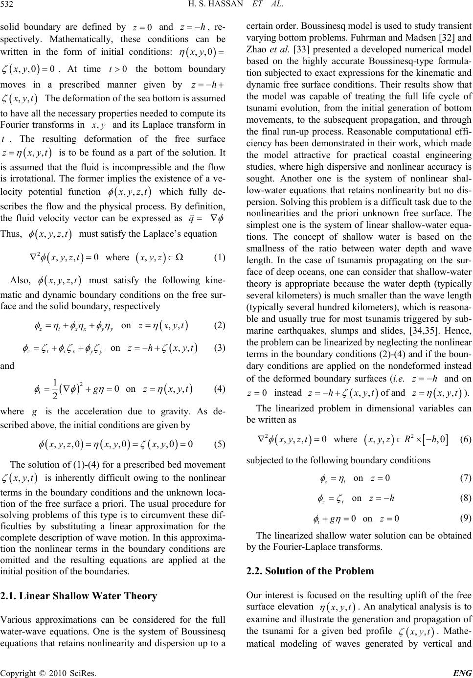

H. S. HASSAN ET AL. 532
solid boundary are defined by 0z and
z
h

, re-
spectively. Mathematically, these conditions can be
written in the form of initial conditions:


,,0xy 



,,0 0xy  . At time 0t the bottom boundary
moves in a prescribed manner given by
z
h




,,
x
yt  The deformation of the sea bottom is assumed
to have all the necessary properties needed to compute its
Fourier transforms in ,
x
y and its Laplace transform in
t. The resulting deformation of the free surface

,,zxyt   is to be found as a part of the solution. It
is assumed that the fluid is incompressible and the flow
is irrotational. The former implies the existence of a ve-
locity potential function

,,,
x
yzt  which fully de-
scribes the flow and the physical process. By definition,
the fluid velocity vector can be expressed as q




Thus,

,,,
x
yzt  must satisfy the Laplace’s equation
 
2,,,0where ,,xyzt xyz
   (1)
Also,

,,,
x
yzt  must satisfy the following kine-
matic and dynamic boundary conditions on the free sur-
face and the solid boundary, respectively

on, ,
ztxxyy zxyt
    (2)


on, ,
ztxxyy zh xyt
    (3)
and
 
2
10on ,,
2
t
g
zxyt     (4)
where
g
is the acceleration due to gravity. As de-
scribed above, the initial conditions are given by

,,,0,,0,,0 0xyz xyxy   (5)
The solution of (1)-(4) for a prescribed bed movement


,,
x
yt  is inherently difficult owing to the nonlinear
terms in the boundary conditions and the unknown loca-
tion of the free surface a priori. The usual procedure for
solving problems of this type is to circumvent these dif-
ficulties by substituting a linear approximation for the
complete description of wave motion. In this approxima-
tion the nonlinear terms in the boundary conditions are
omitted and the resulting equations are applied at the
initial position of the boundaries.
2.1. Linear Shallow Water Theory
Various approximations can be considered for the full
water-wave equations. One is the system of Boussinesq
equations that retains nonlinearity and dispersion up to a
certain order. Boussinesq model is used to study transient
varying bottom problems. Fuhrman and Madsen [32] and
Zhao et al. [33] presented a developed numerical model
based on the highly accurate Boussinesq-type formula-
tion subjected to exact expressions for the kinematic and
dynamic free surface conditions. Their results show that
the model was capable of treating the full life cycle of
tsunami evolution, from the initial generation of bottom
movements, to the subsequent propagation, and through
the final run-up process. Reasonable computational effi-
ciency has been demonstrated in their work, which made
the model attractive for practical coastal engineering
studies, where high dispersive and nonlinear accuracy is
sought. Another one is the system of nonlinear shal-
low-water equations that retains nonlinearity but no dis-
persion. Solving this problem is a difficult task due to the
nonlinearities and the priori unknown free surface. The
simplest one is the system of linear shallow-water equa-
tions. The concept of shallow water is based on the
smallness of the ratio between water depth and wave
length. In the case of tsunamis propagating on the sur-
face of deep oceans, one can consider that shallow-water
theory is appropriate because the water depth (typically
several kilometers) is much smaller than the wave length
(typically several hundred kilometers), which is reasona-
ble and usually true for most tsunamis triggered by sub-
marine earthquakes, slumps and slides, [34,35]. Hence,
the problem can be linearized by neglecting the nonlinear
terms in the boundary conditions (2)-(4) and if the boun-
dary conditions are applied on the nondeformed instead
of the deformed boundary surfaces (i.e.
z
h and on
0z

instead


,,zh xyt   of and


,,zxyt  ).
The linearized problem in dimensional variables can
be written as

 

22
,,,0where ,,,0
x
yztxyz Rh    (6)
subjected to the following boundary conditions
on 0
zt z



 (7)
on
zt zh



 (8)
0on 0
tgz



 (9)
The linearized shallow water solution can be obtained
by the Fourier-Laplace transforms.
2.2. Solution of the Problem
Our interest is focused on the resulting uplift of the free
surface elevation


,,
x
yt

. An analytical analysis is to
examine and illustrate the generation and propagation of
the tsunami for a given bed profile


,,
x
yt

. Mathe-
matical modeling of waves generated by vertical and

H. S. HASSAN ET AL. 533
lateral displacements of ocean bottom using the com-
bined Fourier–Laplace transforms of the Laplace equa-
tion analytically is the simplest way of studying tsunami
development. All our studies took into account constant
depth for which the Laplace and Fast Fourier Transform
(FFT) methods could be applied. Equations (6)-(9) can
be solved by using the method of integral transforms. We
apply the Fourier transform in (x, y) given by


 

12
2 12
ˆ,,
ikxk y
R
f
fkkfxye dxdy



with its inverse transform


 

12
2
1
121 2
2
1
ˆˆ
,,
2
ikxk y
R
f
fxyfkke dkdk




 
and the Laplace transform in time t,
£

 
0
st
g
Gsgte dt



For the combined Fourier and Laplace transforms, the
following notation is introduced
£

12
,,, ,
f
xytF kks


12
20,,
ikxkyst
Redxdyfxytedt

 

Combining (7) and (9) yields the single free-surface
condition



,,0,,,0, 0
tt z
xy tgxy t   (10)
and the bottom condition (8) will be

,, ,,,
zt
x
yht xyt   (11)
The solution of the Laplace Equation (6) which satis-
fies the boundary conditions (10)-(11) can be obtained
by using the Fourier-Laplace transforms method.
First, by applying the transforms method to the Lap-
lace equation (6), gives
F£
  F£   F£    0 (12)
By using the property 
 
nn
n
df ikF k
x




 , (12)
will be






22
121 212
,,,,,, 0
tt kk zskkkk zs
   (13)
Second, by applying the transforms method to the
boundary conditions (10)-(11) and the initial conditions
(5), yields



2
12 12
,,0,,,0, 0
z
skksgkks  
(14)
and


12 12
,,,,,
zkkhsskk s
  (15)
The transformed free-surface elevation can be ob-
tained from (9) as
 
12 12
,, ,,0,
s
kk skks
g
  (16)
The general solution of (13) will be







12 12
12
,,, ,,cosh
,,sinh
kk zsAkk skz
Bk kskz
 
 (17)
where 22
12
kkk . The functions

12
,,
A
kk s and


12
,,Bk ks can be found from the boundary conditions
(14)-(15) as follows
For the bottom condition (at
z
h ):

 
12
,, ,sinh cosh kk hs
A
kkhBkkh
z
 
 
 (18)
Substituting from (18) into (15), yields






12
sinhcosh, ,
A
kkhBk khskks   (19)
For the free surface condition (at 0z):


12
12
,, ,and, ,0, kk hsBkkksA
z
 


 (20)
Substituting from (20) into (14), gives
2
g
k
A
B
s

 (21)
Using (21), (19) can be written as
  
12
2
cosh1tanh, ,
gk
Bkkhkhsk ks
s





(22)
From which,
 
 
12
12 2
,,
,, cosh tanh
gskks
Ak kskhsgkkh




,
 
 
3
12
12 2
,,
,, cosh tanh
skks
Bk kskkhsgkkh




.
Substituting the expressions for the functions


12
,,
A
kk s and


12
,,Bk ks in (17) yields,
 


 
12
12 22
2
,,
,,, cosh
cosh sinh
gskks
kk zskhs
s
kz kz
gk

  




(23)

H. S. HASSAN ET AL. 534
where

tanh
g
kkh   is the circular frequency of
the wave motion.
The free surface elevation

12
,,kk s  can be ob-
tained from (16) as
 


2
12
12 22
,,
,, cosh
skks
kk skh s



 (24)
A solution for


,,
x
yt  can be evaluated for spe-
cified


,,
x
yt  by computing approximately its trans-
form

12
,,kk s  then substituting it into (24) and in-
verting

12
,,kk s  to obtain


,,
x
yt  We are con-
cerned now to evaluate


,,
x
yt  by transforming ana-
lytically the assumed source model then inverting

12
,,kk s  using the inverse Laplace Transform to ob-
tain

12
,,kkt  which is further converted to


,,
x
yt  by using double inverse Fourier Transform.
The circular frequency

describes the dispersion
relation of tsunamis and implies phase velocity ck


and group velocity d Udk

.
Hence,

tanh
g
kh
ck , and

12
1
2sinh2
kh
Uc kh





.
Since, 2 k


, hence as 0kh, both cgh
and Ugh, which implies that the tsunami velocity
t
vgh for wavelengths λ long compared to the water
depth h. The above linearized solution is known as the
shallow water solution. We considered three stages for
the mechanism of the tsunami generation caused by
submarine gravity mass flows, initiated by a rapid curvi-
linear down and uplift faulting with rise time 1 0tt

,
then propagating unilaterally in the positive x-direction
with time 1
ttt

 , to a length L both with finite veloc-
ity v to produce a depletion and an accumulation zones.
The last stage represented by the time variation in the
velocity of the accumulation slide (block slide) moving
in the x-direction with time max ttt
 and decelera-
tion

, where max
t is the maximum time that the slide
takes to stop with minimum deceleration min

. In the
y-direction, the models propagate instantaneously. The
set of physical parameters used in the problem are given
in Table 1.
The first and second stages of the bed motion are
Table 1. Parameters used in the analytical solution of the
problem.
Parameters First stage Second stage
-Source width, W, km 100 100
-Whole width in 1st Stage and
Propagation length in 2nd Stage, km W’ = 100 L = 150
-Water depth (uniform), h, km 2 2
-Acceleration due to gravity,
g, km/sec2 0.0098 0.0098
-Tsunami velocity,
t
vgh, km/sec 0.14 0.14
-Moving velocity, v, km/sec 0.14 0.14
-Duration of the source process,
t, min 1
50 5.95tv
 200 23.8tv

shown in Figures 2 and 3, respectively, and given by:
1) First Stage: Curvilinear down and Uplift Faulting




down
0
0
0
,,
1 cos1cos150,
250 100
5050, 15050,
1cos ,
50
5050, 5050,
1 cos1 cos50,
250100
5050, 50150.
xyt
vt xy
W
xy
vt x
W
xy
vt xy
W
xy








 
 
 


 

 





 

 
 



 



(25)


 

 
up
0
0
0
,,
1 cos2001cos150,
2 50100
200300, 15050,
1 cos200,
50
200300, 5050,
1 cos2001cos50,
250 100
200300,50150.
xyt
vt xy
W
xy
vt x
W
xy
vt xy
W
xy








 
 
 
 

 





 


 



 



(26)
For these displacements, the bed rises during 1 0tt


to a maximum displacement 0

such that the volume of

H. S. HASSAN ET AL. 535
(a)
(b)
Figure 2. Normalized bed deformation represented by a
rapid curvilinear down and uplift faulting at the end of
stage one (150
tv )(a) Side view along the axis of symmetry
at 0y (b) Three- dimensional view.
(a)
(b)
Figure 3. Normalized Bed deformation model represented
by the accumulation and deplet ion zones at the end of stage
two (200
tv ) (a) Side view along the axis of symmetry at
0y (b) Three-dimensional view.
soil in the uplift increases linear with time and vise verse
in the down faulting.
For 1 tt the soil further propagates unilaterally in
the positive x-direction with velocity v till it reaches the
characteristic length L = 150 km at 200tt v

 .
2) Second Stage: Curvilinear down and Uphill
Slip-Fault (Slump and the Slide)





down1down 2down
3down
,,,, ,,
,,
x
ytxyt xyt
xyt



 (27)
where,





  
 
1down
0
0
1
0
1
11
,,
1 cos1cos150,
450 100
500, 15050,
1 cos150,
2 100
0, 15050,
1 cos1 cos150,
450 100
50, 15050.
xyt
xy
xy
y
xttv y
xttv y
ttv xttvy





 
 


 

 

 



 


















 
2down
0
0
1
0
1
11
,,
1cos ,
250
500, 5050,
,
0, 5050,
1cos ,
250
50, 5050.
xyt
x
xy
xttv y
xttv
ttv xttvy







 

 


 


  


 






  
 
3down
0
0
1
0
1
11
,,
1 cos1 cos50,
4 50100
500,50150,
1 cos50,
2100
0,50150,
1 cos1 cos50,
450 100
50, 50150.
xyt
xy
xy
y
xttvy
xttvy
ttv xttvy





 



 



 



 



 
 


 

 

 





up1up 2up3up
,,,, ,, ,,
x
ytxytxyt xyt   (28)

H. S. HASSAN ET AL. 536
By referring to Figure 3,

1up ,,
x
yt  ,


2up ,,
x
yt 
and

3up ,,
x
yt  can be expressed in the same manner
as


1down ,,
x
yt 


2down ,,
x
yt  and


3down ,,
x
yt  .
The kinematic realistic tsunami source model shown
in Figure 3 is initiated by a rapid curvilinear down and
uplift faulting (First stage) which then spreads unilate-
rally with constant velocity v causing a depletion and
accumulation zones. The final down lift of the depression
zone and final uplift of the accumulation zone are as-
sumed to have the same amplitude 0

. We assume the
spreading velocity v of the slump and the slide deforma-
tion in Figure 3 the same as the tsunami wave velocity
t
vgh as the largest amplification of the tsunami
amplitude occurs when t
vv due to wave focusing
[6,36]. The slide and the slump are assumed to have con-
stant width W.
The spreading is unilateral in the x-direction as shown
in Figure 3. The vertical displacement, 0

, is negative
(downwards) in zones of depletion, and positive (up-
wards) in zones of accumulation. All cases are characte-
rized by sliding motion in one direction, without loss of
generality coinciding with the x-axis, and tsunami prop-
agating in the x-y plane.
Figure 4 shows vertical cross-sections (through y = 0)
of the mathematical models of the stationary submarine
slump and the moving slide and their schematic repre-
sentation of the physical process that we considered in
this study, as those evolve for time tt

. The block
slide starts moving in the positive x-direction at time
tt

 and stops moving at distance 150L km while
the downhill slide becomes stationary. We discuss the
tsunami generation for two cases of the movement of the
block slide. First, the limiting case in which the block
slide moves with constant velocity v and stops after dis-
tance
L
 with infinite deceleration (sudden stop) at time
min
ttLv

 . Second, the general case in which the
block slide moves in time 2
tt

. With constant veloci-
ty and then with constant deceleration such that it stops
softly after traveling the same distance
L
 in time 3
t
which depends on the deceleration

and the choice of
time 2 t. The variation of the ‘‘block slide’’ we consi-
dered could be used to represent the motion of the col-
lapsed blocks at the Blake Escarpment, east of Florida.
(see Figure 7 in Dillon et al. [37]) and the block slide at
the base of Middle Canyon along the Beringian Margin
in Alaska (see Figure 8 in Carlson et al. [38]) and the
Sur submarine landslide originated on the continental
slope west of Point Sur, central California(see Figure 1
in Gutmacher and Normark [39]). So, the evidence of a
huge historical tsunami needs for investigating the possi-
bility of future tsunami generating by submarine land-
slides.
The velocity


vt in this case can be defined as
 
2
22 3
vttt
vt vttt tt








 (29)
where 0.14
t
vv

 km/sec and

is the deceleration
of the moving block slide. We need to determine the time
3
t that the slide takes to reach the final distance
L

and
(a)
v(t)
Displaced
L'
Landslide scar
Landslide scar
(b)
Displaced
v(t)
L'
L
L
Landslide scar
(c)
Figure 4. A schematic representation of a landslide (bottom)
travelling a significant distance L downhill creating a “scar”
and a moving uphill displaced block slide stopping at the
characteristic length

L. (a) Case 1: Mathematical model
of the stationary slump and the moving submarine slide; (b)
Case 2: Physical process of the displaced block moving with
a variable slide velocity


vt; (c) Case 3: Schematic repre-
sentation of the used model.

H. S. HASSAN ET AL. 537
the corresponding deceleration

. This can be done by
the following steps:
1) Choosing time 2 t as

2
ttt Lv


 in
which the slide moves with constant velocity v where
1
ttLv
 and 150tv.
2) Getting the corresponding distance


2
L
ttv

 .
3) Evaluating the remaining distance

2
L
Lttv
 

 .
Substituting
L
 n the equation

2
32 32
1
2
L
ttv tt
  (30)
When the block slide stops moving, then





3232 0vtv t t t t  (31)
Eliminating

from (30) and (31), we get a relation
between 3 t and 2 t which further on substituting in
(31), we obtain the deceleration

.
For 23 ttt , the block slide moves with velocity

2
vtvt t

 . Table 2 represents the different
Table 2. Values of 2 t and the corresponding calculated
values of 3
tand

.
Time t2 (minutes) Time t3 (minutes) Deceleration α
t* = 23.80 59.51 6.53 × 10-5
t* + 0.1(L’/v) = 25.58 57.72 7.25 × 10-5
t* + 0.2(L’/v) = 27.37 55.95 8.16 × 10-5
t* + 0.3(L’/v) = 29.37 54.15 9.33 × 10-5
t* + 0.4(L’/v) = 30.94 52.36 1.08 × 10-4
t* + 0.5(L’/v) = 32.72 50.57 1.30 × 10-4
t* + 0.6(L’/v) = 34.51 48.79 1.63 × 10-4
t* + 0.7(L’/v) = 36.30 47.01 2.17 × 10-4
t* + 0.8(L’/v) = 38.08 45.22 3.26 × 10-4
t* + 0.9(L’/v) = 39.87 43.44 6.53 × 10-4
t* + (L’/v) = 41.65 41.65 infinity
values of 2 t and the corresponding calculated values of
3
t and

.
Figure 5 illustrates the position of the slides in the
third stage for different choice of deceleration

. In this
stage, min

is the minimum deceleration required such
that the slide stops after traveling distance
L
.
In this case 2 tt


and


3max 2tt tLv

 
59.51min . For any other min

 , the slide moves with
constant velocity with time 2 ttt
 and with decele-
ration

until it stops at time 3 t which is less than
max
t.
So, the stationary landslide scar for tt
 and the
movable block slide with variable velocity


vt for


2
ttt Lv


 and



32tLvtt Lv


 
can be expressed respectively as







stat.landslide1 2
3
,, ,, ,,
,,
x
yt xyt xyt
xyt






 (32)

  

block slide12
3
,, ,, ,,
,,
x
yt xyt xyt
xyt



 (33)


stat.landslide ,,
x
yt 

is the same as (27) except the time
parameter t will be substituted by t.
For


block slide,,
x
yt  , let η(x,0,t)
Figure 5. Slide block position against the instants of times





2
ttt Lv and 
min3 max
ttt
.

H. S. HASSAN ET AL. 538



2
2
223
for
1for
2
ttvtt t
S
ttvtttt t





 


be the distance the slide moves during stage three, hence


  




1
0
0
0
,,
1 cos2001 cos150,
450 100
200250,15050,
1cos150 ,
2100
250250, 15050,
1 cos2501 cos150,
450 100
250300, 150
xyt
xS y
Sx Sy
y
Sx SLy
xSL y
SLx SLy






 








  

 


 50.
















 


2
0
0
0
,,
1 cos200,
250
200250, 5050,
,
250250, 5050,
1 cos250,
250
250300, 5050.
xyt
xS
Sx Sy
Sx Sy
xSL
SLx SLy










 


 






 



  

  
3
0
0
0
,,
1 cos2001 cos150,
450 100
200250, 50150,
1 cos150,
2100
250250, 50150,
1 cos2501 cos150,
450 100
250300, 50150.
xyt
xS y
SxS y
y
SxSL y
xSL y
SLxSL y






 



 




 

 
 

 

 
 














Laplace and Fourier transforms can now be applied to
the bed motion described by (25)-(28) and (32)-(33).
First, beginning with the down and uplift faulting (25)
and (26) for 1 0tt

 where 1
50
tv , and
£




12
,,, ,
x
ytk ks  


12
0,,
ikxk yst
edxdyxytedt 

 

 (34)
The limits of the above integration are apparent from
(25)-(26).
Substituting the results of the integration (34) for
down

and up

into (24). The free surface elevation


12
,,kkt  can be evaluated by using the inverse Lap-
lace transforms of


12
,,kks  . From which,
 


11
11
11
11
2
200 300
300 200
1
2
1
1
0
12
2
50 50
50 50
1
2
1
1
150
50
1
sin
,, cosh 2
150
50
1
ik ik
ik ik
ik ik
ik ik
ee ike e
ik k
v t
kkt kh W
ee ike e
ik k


 



 














 


















 










22
22
22
22
2
150 50
2
50 150
2
2
2 2
2
2
50 150
150 50
2
2
2
2
4sin50
1100
100
1
1 100
100
1
ik ik
iki k
ikik
ik ik
k
ee ikee
ik k
k
ee ike e
ik k




 























 











 




 



















(35)

H. S. HASSAN ET AL. 539
In case of 1 tt,

12
,,kkt  will have the same ex-
pression except in the convolution step, the integral be-
comes

1
0
sin
sin
cos
ttt
t
d


 


 instead of
0
sin
cos
tt
d

 


.
Finally,


,,
x
yt  is evaluated using the double in-
verse Fourier transform of


12
,,kkt 

 
21
1212
2
1
,,, ,
2
ikyik x
x
yteekkt dkdk 


 




(36)
This inversion is computed by using the FFT. The in-
verse FFT is a fast algorithm for efficient implementa-
tion of the Inverse Discrete Fourier Transform (IDFT)
given by
 
22
11
00
1
,,,
0,1, ,1,0,1,1,
MN ipmiqn
MN
pq
fmnFpqe e
MN
pMqN

 
 
 





where


,
f
mn is the resulting function of the two spa-
tial variables m and n, corresponding to x and y, from the
frequency domain function


,
F
pq with frequency
variables p and q, corresponding to k1 and k2. This inver-
sion is done efficiently by using the Matlab FFT algo-
rithm.
Using the same steps,


12
,,kkt  is evaluated by ap-
plying the Laplace and Fourier transforms to the bed
motion described by (27) and (28), then substituting into
(24) and then inverting

12
,,kk s  using the inverse
Laplace transform to obtain

12
,,kkt  . This is verified
for 1 ttt


 where 200 tv
 as




1 2down12up1 2
,,,, ,,kktkkt kkt    (37)
where,





down 121down 122down 12
3down1 2
,,,,,,
,,
kktkkt kkt
kkt




then
and





up1 21up1 22up1 2
3up1 2
,,,,,,
,,
kktkkt kkt
kkt




then






22
22
22
2
150 50
50 150
0
2
2
2
2
2
0
down1 2
2
50 150
0
2
2
1 100
4cosh 100
1
sin 50
,, cosh
1
4cosh 100
1
ik ik
ikik
iki k
ee ike e
kh ikk
k
kkt khk
ee
kh ikk














 

 


 

 
 














 

 
 




 
22
11
1
2
150 50
2
2
2
50 50
50
11
2
1
1
11 1
2
2
1
100
150
1cos
50
1
2sin
ik ik
ik ik
ik
ike e
ee
iket t
ik k
vttikv tt
kv




 



 
 
 
 
 
 
 
 
 
 
 

 



 




 




 


 


 










 






 



   
   


11
1111
11 11
1
2
50
50
1 1
2
1
1
150
1cos
50
1
ikt tv
ikt tvikt tv
ikt tvikt tv
ik ve
ee ikeet t
ik k




  
 
 
 
 
 
 
 
 

 
 
 
 
 
 

 

 


  
 

 

 

 

 

 
 

H. S. HASSAN ET AL. 540






22
22
22
2
150 50
50 150
0
2
2
2
2
2
0
up1 2
2
50 150
0
2
2
2
1100
4cosh 100
1
sin 50
,, cosh
1
4cosh 100
1
ik ik
iki k
iki k
ee ike e
kh ikk
k
kkt kh k
ee
kh ikk










 




 


 

 















 

 
 





22
11
11
1
2
150 50
2
2
200 250
250 200
11
2
1
1
250
2
2
1
100
150cos
50
1
2
ik ik
ik ik
ik ik
ik
ike e
ee ikeet t
ik k
ve
kv







 

 
 
 
 
 
 
 
 
 
 
 

 



 




 




 

 

 





 




 








 












11
11 11
11 11
11 11
2
250 300
300 250
1
2
1
1
1
sin cos
150
50
1
cos
ikt tv
ikttvikt tv
ikt tvikt tv
tt ikvttikve
ee ik ee
ik k
tt





 
 
 
 
 
 
 
 
 
 
 
 
 
 
 
 



 
 




 
 


 


 

 

 

 
 

 
Substituting


down1 2
,,kkt  and

up1 2
,,kkt  into
(37) gives


12
,,kkt  for 1 ttt

 . For the case
tt

,


12
,,kkt  will have the same expression as (37)
except for the term resulting from the convolution theo-
rem, i.e.




 





11
1
1
2
2
1
111
11 1
1
cos
sin cos
sin cos
tikt tv
tt t
ik vt
ed
kv
tt ikvtt e
tt tikvtt t

 
 
 








 


 


,
instead of



 


11
1
11
2
2
1
11 11
1
cos
sin cos
tik t tv
tt
ik vttv
ed
kv
tt ikvtt ikve
 
 




 
.
So,


,,
x
yt  is computed using inverse FFT of


12
,,kkt  .
Finally,

block slide12
,,kkt  is evaluated by applying
the Laplace and Fourier transforms to the block slide
motion described by (33), then substituting into (24) and
then inverting


block slide12
,,kk s  using the inverse
Laplace transform to obtain

block slide12
,,kkt  . This is
verified for


2
tttLv

  and


3
tLvt




2tLv


 . Then,



block slide12112212
312
,, ,, ,,
,,
kkt kkt kkt
kkt



 (38)
Then,
Finally,


,,
x
yt  is computed using inverse FFT of


12
,,kkt  .
We investigated mathematically the water wave mo-
tion in the near and far-field by considering a kinematic
mechanism of the sea floor faulting represented in se-
quence by a down and uplift motion with time followed
by unilateral spreading in x-direction, both with constant
velocity v, then a deceleration movement of a block
slide in the direction of propagation. Clearly, from the
mathematical derivation done above,


,,
x
yt

de-
pends continuously on the source


,,
x
yt  . Hence,
from the mathematical point of view, this problem is said
to be well-posed for modeling the physical processes of
the tsunami wave.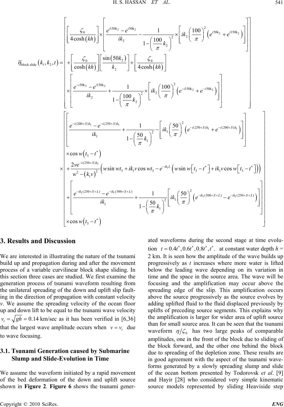

H. S. HASSAN ET AL. 541






22
22
22
2
150k 50k
50k 150k
0
2
2
2
2
2
00
block slide12
2
50k 150k
2
2
1100
4cosh 100
1
sin 50
,, cosh 4cosh
1
100
1
ii
ii
ii
ee ike e
kh ikk
k
kkt kh kkh
ee
ik k













 

 


 

 





 
 



 





22
11
11
2
150k50k
2
2
2
(200 )(250 )
(250 )(200 )
1
2
1
1
100
150
50
1
cos
ii
iSk iSk
iSk iSk
ike e
ee ikee
ik k




  
























 













 




 

 










1
1
11
11
3
(250 )
31 3313
2
2
1
2
(250 )(300)
(300 )(250 )
1
2
1
1
2sin cossincos
150
50
1
cos
iSk
ik L
ikS LikS L
ikS LikS L
wt t
ve wwtikvwtewwt tikvwt t
wkv
ee ik ee
ik k 


 
 

 

 










 







 











3
wt t

 
 
 
 
 
 
 
 
 
 
 
 
 
 
 
 
 
 
 
 

 
3. Results and Discussion
We are interested in illustrating the nature of the tsunami
build up and propagation during and after the movement
process of a variable curvilinear block shape sliding. In
this section three cases are studied. We first examine the
generation process of tsunami waveform resulting from
the unilateral spreading of the down and uplift slip fault-
ing in the direction of propagation with constant velocity
v. We assume the spreading velocity of the ocean floor
up and down lift to be equal to the tsunami wave velocity
0.14
t
vghkm/sec as it has been verified in [6,36]
that the largest wave amplitude occurs when t
vv

due
to wave focusing.
3.1. Tsunami Generation caused by Submarine
Slump and Slide-Evolution in Time
We assume the waveform initiated by a rapid movement
of the bed deformation of the down and uplift source
shown in Figure 2. Figure 6 shows the tsunami gener-
ated waveforms during the second stage at time evolu-
tion 0.4,0.6,0.8,.ttttt


 at constant water depth h =
2 km. It is seen how the amplitude of the wave builds up
progressively as t increases where more water is lifted
below the leading wave depending on its variation in
time and the space in the source area. The wave will be
focusing and the amplification may occur above the
spreading edge of the slip. This amplification occurs
above the source progressively as the source evolves by
adding uplifted fluid to the fluid displaced previously by
uplifts of preceding source segments. This explains why
the amplification is larger for wider area of uplift source
than for small source area. It can be seen that the tsunami
waveform 0

 has two large peaks of comparable
amplitudes, one in the front of the block due to sliding of
the block forward, and the other one behind the block
due to spreading of the depletion zone. These results are
in good agreement with the aspect of the tsunami wave-
forms generated by a slowly spreading slump and slide
of the ocean bottom presented by Todorovsk et al. [9]
and Hayir [28] who considered very simple kinematic
source models represented by sliding Heaviside step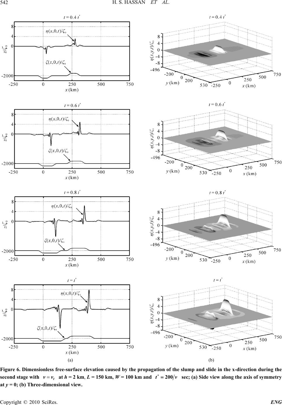

H. S. HASSAN ET AL. 542
(a) (b)
Figure 6. Dimensionless free-surface elevation caused by the propagation of the slump and slide in the x-direction during the
second stage with t
vv
at h = 2 km, L = 150 km, W = 100 km and 200tv sec; (a) Side view along the axis of symmetry
at y = 0; (b) Three-dimensional view.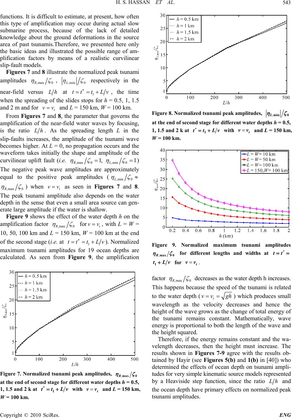

H. S. HASSAN ET AL. 543
functions. It is difficult to estimate, at present, how often
this type of amplification may occur during actual slow
submarine process, because of the lack of detailed
knowledge about the ground deformations in the source
area of past tsunamis.Therefore, we presented here only
the basic ideas and illustrated the possible range of am-
plification factors by means of a realistic curvilinear
slip-fault models.
Figures 7 and 8 illustrate the normalized peak tsunami
amplitudes ,max0R

, ,min0L

 respectively in the
near-field versus
L
h at 1 ttt Lv

 , the time
when the spreading of the slides stops for h = 0.5, 1, 1.5
and 2 m and for t vv and L = 150 km, W = 100 km.
From Figures 7 and 8, the parameter that governs the
amplification of the near-field water waves by focusing,
is the ratio
L
h. As the spreading length L in the
slip-faults increases, the amplitude of the tsunami wave
becomes higher. At L = 0, no propagation occurs and the
waveform takes initially the shape and amplitude of the
curvilinear uplift fault (i.e. ,max0,min 0 1, 1
RL
 
 )
The negative peak wave amplitudes are approximately
equal to the positive peak amplitudes (,min 0L


,max0R

) when t vv as seen in Figures 7 and 8.
The peak tsunami amplitude also depends on the water
depth in the sense that even a small area source can gen-
erate large amplitude if the water is shallow.
Figure 9 shows the effect of the water depth h on the
amplification factor ,max 0R

fort vv, with L = W =
10, 50, 100 km and L = 150 km, W = 100 km at the end
of the second stage (i.e. at 1 ttt Lv

 ). Normalized
maximum tsunami amplitudes for 19 ocean depths are
calculated. As seen from Figure 9, the amplification
Figure 7. Normalized tsunami peak amplitudes, ,max0R

at the end of second stage for different water depths h = 0.5,
1, 1.5 and 2 k at 1 ttLv with t vv and L = 150 km,
W = 100 km.
Figure 8. Normalized tsunami peak amplitudes, ,min 0L


at the end of second stage for different water depths h = 0.5,
1, 1.5 and 2 k at 1
ttLv with t
vv
and L = 150 km,
W = 100 km.
Figure 9. Normalized maximum tsunami amplitudes
,max 0R

for different lengths and widths at  tt


1
tLv

for

t
vv .
factor ,max0R

decreases as the water depth h increases.
This happens because the speed of the tsunami is related
to the water depth (t vv gh ) which produces small
wavelength as the velocity decreases and hence the
height of the wave grows as the change of total energy of
the tsunami remains constant. Mathematically, wave
energy is proportional to both the length of the wave and
the height squared.
Therefore, if the energy remains constant and the wa-
velength decreases, then the height must increase. The
results shown in Figures 7-9 agree with the results ob-
tained by Hayir (see Figures 5(b) and 1(b) in [40]) who
determined the effects of ocean depth on tsunami ampli-
tudes for very simple kinematic source models represented
by a Heaviside step function, since the ratio
L
h and
the ocean depth have primary effects on normalized peak
tsunami amplitudes.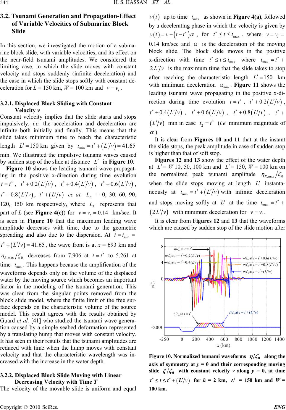

H. S. HASSAN ET AL. 544
3.2. Tsunami Generation and Propagation-Effect
of Variable Velocities of Submarine Block
Slide
In this section, we investigated the motion of a subma-
rine block slide, with variable velocities, and its effect on
the near-field tsunami amplitudes. We considered the
limiting case, in which the slide moves with constant
velocity and stops suddenly (infinite deceleration) and
the case in which the slide stops softly with constant de-
celeration for L = 150 km, W = 100 km and t
vv.
3.2.1. Displaced Block Sliding with Constant
Velocity v
Constant velocity implies that the slide starts and stops
impulsively, i.e. the acceleration and deceleration are
infinite both initially and finally. This means that the
slide takes minimum time to reach the characteristic
length 150Lkm given by

min 41.65ttLv


min. We illustrated the impulsive tsunami waves caused
by sudden stop of the slide at distance
L
 in Figure 10.
Figure 10 shows the leading tsunami wave propagat-
ing in the positive x-direction during time evolution
tt

,


0.2tLv

,


0.4tLv

,


0.6tLv


,


0.8tLv

,


tLv

 ec at.
E
L
= 0, 30, 60, 90,
120, 150 km respectively, where
E
L
represents that
part of L (see Figure 4(c)) for 0.14
t
vv km/sec. It
is seen in Figure 10 that the maximum leading wave
amplitude decreases with time, due to the geometric
spreading and also due to the dispersion. At min tt



41.65tLv

 , the wave front is at x = 693 km and
,max0R

decreases from 7.906 at tt

 to 5.261 at
time mi n t. This happens because the amplification of the
waveforms depends only on the volume of the displaced
water by the moving source which becomes an important
factor in the modeling of the tsunami generation. This
was clear from the singular points removed from the
block slide model, where the finite limit of the free sur-
face depends on the characteristic volume of the source
model. This result agrees with the results obtained by
Guard et al. [41] who studied the tsunami wave genera-
tion caused by a simple seabed deformation represented
by a translating hump that moves with constant velocity.
It has seen in their results that the tsunami amplitudes are
reduced with time when the hump moves with constant
velocity and that the characteristic wavelength was in-
creased with the increase in the water depth.
3.2.2. Displaced Block Slide Moving with Linear
Decreasing Velocity with Time T
The velocity of the movable slide is uniform and equal


vt up to time max t as shown in Figure 4(a), followed
by a decelerating phase in which the velocity is given by




vtvt t


 , for max ttt
 . where t
vv


0.14 km/sec and

is the deceleration of the moving
block slide. The block slide moves in the positive
x-direction with time max ttt
 where max
tt



2
L
v

is the maximum time that the slide takes to stop
after reaching the characteristic length 150L

km
with minimum deceleration min

. Figure 11 shows the
leading tsunami wave propagating in the positive x-di-
rection during time evolution tt

,


0.2tLv


,


0.4tLv


,


0.6tLv

,


0.8tLv

, t



Lv

min in case 2 tt


(i.e. minimum magnitude of

).
It is clear from Figures 10 and 11 that at the instant
the slide stops, the peak amplitude in case of sudden stop
is higher than that of soft stop.
Figures 12 and 13 show the effect of the water depth
at
L

= W 10, 50, 100 km and
L
= 150, W = 100 km on
the normalized peak tsunami amplitude ,max 0R

when the slide stops moving at length
L

instanta-
neously at


min
ttLv


 with infinite deceleration
and stops moving softly at
L
 at the time max
tt





2Lv

with minimum deceleration for t vv.
It is clear from Figures 12 and 13 that the waveforms
which are caused by sudden stop of the slide motion after
Figure 10. Normalized tsunami waveforms 0

 along the
axis of symmetry at y = 0 and their corresponding moving
slide 0


with constant velocity v along y = 0, at time




tttLv  for h = 2 km,  L = 150 km and W =
100 km.

H. S. HASSAN ET AL. 545
Figure 11. Normalized tsunami waveforms 0

 and their
corresponding moving slide 0

 with variable velocity

vt along y = 0, at time



2ttt Lv  at h = 2 km,

L = 150 km and W = 100 km.
Figure 12. Normalized maximum tsunami amplitudes
,max 0

R when the slide stops suddenly at time min
t



tLv with different slide lengths L and widths W and
for t vv.
they reach the characteristic length
L
 at time min
t



tLv

 have higher amplitude than stopping of the
slide with slow motion at time 

max 2tt Lv


 . This
agrees with the mathematical relation between the wave-
length and the wave height where the wave energy is
proportional to both the length of the wave and the
height squared.
3.2.3. Displaced Block Slide Moving with Constant
Velocity v Followed by Variable Velocity


vt
In this section, we studied the generation of the tsunami
waveforms when the block slide moves a significant dis-
tance with constant velocity t vv

then continues moving
Figure 13. Normalized maximum tsunami amplitudes
,max 0

R when the slide stops softly at time max
t





2tLv with different slide lengths L and widths W
and for t
vv

.
with variable velocity


vt with constant deceleration
until it stops at the characteristic length
L
 = 150 km.
Figure 14 shows the tsunami waveforms at the times
calculated in Table 2 when the slide reaches the charac-
teristic length
L

= 150 km.
In Figure 14, the blue waveform indicates the shape
of the wave at the time

3min 41.65ttt Lv


min in the limiting case when the slide stops moving
suddenly. The green waveform indicates the wave in the
other limiting case at the time


3max 2tt tLv



when the slide stops moving with minimum deceleration
at the distance
L

. In between the two limiting cases, the
slide begins moving with constant velocity a significant
distance followed by decelerating movement until it
stops at the characteristic length
L
 = 150 km at the
time min3 max
ttt

, see Table 2. It is seen how the peak
amplitudes of the leading waves decreases gradually
from 5.261 to 3.894.
In order to compare the shape and maximum height of
tsunami wave at certain time for different deceleration

, we choose the time max tt

. For the limiting case
min

, there is no free propagation, while for the other
limiting case “the sudden stop”, there is maximum free
propagation between time min t and max t. For the cases
between the two limiting cases, the propagation time is
p
ropmax 3
ttt

.
Figure 15 shows the shape of the tsunami propagation
waveform at


max 259.51ttLv

 min (curves in
black) for different deceleration

and time 3 t (time
at which the slide stops). As the wave propagates, the
wave height decreases and the slope of the wave front

H. S. HASSAN ET AL. 546
Figure 14. Normalized tsunami waveforms 0

 along y =
0 at 3 tt calculated in Table 2 with 
L = 150 km.
becomes smaller, causing a train of small wave forms
behind the main wave. The maximum wave amplitude
decreases with time, due to the geometric spreading and
also due to the dispersion.
Figure 16 represents the normalized peak tsunami
amplitudes 0
min

and max 0

 of the leading
propagating wave in the far-field at the time max
tt

for
the different deceleration

and time 3 t (time at
which the slide stops) chosen in Figure 15.
Figure 15. Normalized tsunami propagation waveforms
0

 along the axis of symmetry at y = 0 at time max t =
59.51 min and at time 3
t for different deceleration

.

H. S. HASSAN ET AL. 547
Figure 16. The normalized peak tsunami amplitudes
0
min

 and max 0

 at time max tt for the different
deceleration

and time 3 t.
It can be seen in Figure 16 that the absolute minimum
peak amplitudes of the leading propagated waves at time

max 2ttLv

 , after the block slide stops moving
with different deceleration

and time 3
t, decrease
gradually, while the maximum peak amplitudes increase
progressively.
4. Conclusions
In this paper, we presented a review of the main physical
characteristics of the tsunami generation caused by rea-
listic curvilinear submarine slumps and slides in the
near-field. It is seen that the tsunami waveform has two
large peaks of comparable amplitudes, one in the front of
the block due to forward sliding of the block, and the
other one behind the block due to spreading of the deple-
tion zone. The negative peak wave amplitudes are ap-
proximately equal to the positive peak amplitudes. These
results agree with the qualitative behaviour of the tsuna-
mi waveforms generated by a slowly spreading slump
and slide of the ocean bottom presented by Todorovsk et
al. [9] and Hayir [28] who considered very simple kine-
matic source models represented by sliding Heaviside
step functions. We studied the effect of variable veloci-
ties of submarine block slide on the tsunami generation
in the limiting cases, in which the slide moves with con-
stant velocity and stops suddenly (with infinite decelera-
tion) and the case in which the slide stops softly at the
same place with minimum deceleration. It is seen that the
leading tsunami amplitudes are reduced in both cases due
to the geometric spreading and also due to the dispersion.
We observed that the peak tsunami amplitudes increase
with the decrease in the sliding source area and the water
depth. We also investigated the more realistic case in
which the block slide moves a significant distance with
constant velocity v then continue moving with time de-
pendence velocity


vt and different constant decelera-
tion until it stops at the characteristic length. It is seen
how the peak amplitudes of the leading waves decrease
gradually with time between the two limiting cases. In
this case we demonstrated also the shape of tsunami
propagated wave at certain time max t (time at which the
slide stops with minimum deceleration). The results
show that the wave height decreases due to dispersion
and the slope of the front of the wave becomes smaller,
causing a train of small wave forms behind the main
wave. It can be observed that just a slight variation in the
maximum and the minimum tsunami propagated ampli-
tudes after the block slide stops moving with different
deceleration

and time 3 t, see Figure 16. The pre-
sented analysis suggests that some abnormally large tsu-
namis could be explained in part by variable speeds of
submarine landslides. Our results should help to enable
quantitative tsunami forecasts and warnings based on
recoverable seismic data and to increase the possibilities
for the use of tsunami data to study earthquakes, particu-
larly historical events for which adequate seismic data do
not exist.
5. Acknowledgments
The authors would like to express their gratitude to Pro-
fessor Mina B. Abd-el-Malek, head of the Department of
Engineering Mathematics and Physics, Faculty of Engi-
neering, Alexandria University, Egypt for his valuable
suggestions and discussions which led to many im-
provements of the manuscript. The authors would like to
thank the reviewer for his/her valuable comments, which
improved the paper.
6. References
[1] M. S. Abou-Dina and F. M. Hassan, “Generation and
Propagation of Nonlinear Tsunamis in Shallow Water by
a Moving Topography,” Applied Mathematics and Com-
putation, Vol. 177, No. 2, 2006, pp. 785-806.
[2] F. M. Hassan, “Boundary Integral Method Applied to the
Propagation of Non-linear Gravity Waves Generated by a
Moving Bottom,” Applied MathematicalModelling, Vol.
33, No. 1, 2009, pp. 451-466.
[3] N. Zahibo, E. Pelinovsky, T. Talipova , A. Kozelkov and
A. Kurkin, “Analytical and Numerical Study of Nonlinear
Effects at Tsunami Modeling,” Applied Mathematics and
Computation, Vol. 174, No. 2, 2006, pp. 795-809.
[4] K. Das, S. Green, D. Basu, R. Janetzke and J. Stamatakos,
“Effect of Slide Deformation and Geometry on Waves
Generated by Submarine Landslides: A Numerical Inves-
tigation,” Offshore Technology Conference, Texas, USA,
May 2009, pp. 1-12.
[5] Ben-Menahem and M. Rosenman, “Amplitude Patterns

H. S. HASSAN ET AL. 548
of Tsunami Waves from Submarine Earthquakes,” Jour-
nal of Geophysical Research, Vol. 77, No. 17, 1972, pp.
3097-3128.
[6] M. I. Todorovska and M. D. Trifunac, “Generation of
Tsunamis by a Slowly Spreading Uplift of the Sea Floor,”
Soil Dynamics and Earthquake Engineering, Vol. 21, No.
2, 2001, pp. 151-167.
[7] M. D. Trifunac and M. I. Todorovska, “A Note on Dif-
ferences in Tsunami Source Parameters for Submarine
Slides and Earthquakes,” Soil Dynamics and Earthquake
Engineering, Vol. 22, No. 2, 2002, pp.143-155.
[8] M. D. Trifunac, A. Hayir and M. I. Todorovska, “A Note
on Tsunami Caused by Submarine Slides and Slumps
Spreading in One Dimension with Nonuniform Dis-
placement Amplitudes,” Soil Dynamics and Earthquake
Engineering, Vol. 23, No. 3, 2003, pp. 223-234.
[9] M. I. Todorovsk, M. D. Trifunac and A. Hayir, “A Note
on Tsunami Amplitudes above Submarine Slides and
Slumps,” Soil Dynamics and Earthquake Engineering,
Vol. 22, No. 2, 2002, pp. 129-141.
[10] M. D. Trifunaca, A. Hayira and M. I. Todorovska, “Was
Grand Banks Event of 1929 a Slump Spreading in Two
Directions,” Soil Dynamics and Earthquake Engineering,
Vol. 22, No. 5, 2002, pp. 349-360.
[11] Hayir, “The Near-Field Tsunami Amplitudes Caused by
Submarine Landslides and Slumps Spreading in Two
Prthogonal Directions,” Ocean Engineering, Vol. 33, No.
5-6, 2006, pp. 654-664.
[12] S. A. Beisel, L. B. Chubarov, Z. I. Fedotova and G. S.
Khakimzyanov, “On the Approaches to a Numerical
Modeling of Landslide Mechanism of Tsunami Wave
Generation,” Communications in Applied Analysis, Vol.
11, No. 1, 2007, pp. 121-135.
[13] P. Lynett and L.-F. Liu Philip, “A Numerical Study of
Submarine-Landslide-Generated Waves and Run-Up,”
Proceeding of the Royal Society A, Vol. 458, No. 2028,
2002, pp. 2885-2910.
[14] L. Jiang and P. H. Le Blond, “The Coupling of a Subma-
rine Slide and the Surface Waves Which it Generates,”
Journal of Geophysical Research, Vol. 97, No. C8, 1992,
pp. 12731-12744.
[15] S. Rzadkiewicz, C. Mariotti and P. Heinrich, “Numerical
Simulation of Submarine Landslides and Their Hydraulic
Effects,” Journal of Waterway, Port, Coastal, and Ocean
Engineering, Vol. 123, No. 4, 1997, pp. 149-157.
[16] S. T. Grilli and P. Watts, “Modeling of Waves Generated
by a Moving Dubmerged Body, Applications to Under-
water Landslides,” Journal of Engineering Analysis with
Boundary Elements, Vol. 23, No. 8, pp. 1999, 645-656.
[17] P. Watts, S. T. Grilli, D. R. Tappin and G. J. Fryer,
“Tsunami Generation by Dubmarine Mass Failure. II:
Predictive Equations and Case Studies,” Journal of Wa-
terway, Port, Coastal, and Ocean Engineering, Vol. 131,
No. 6, 2005, pp. 298-310.
[18] B. Ataie-Ashtiani and G. Shobeyri, “Numerical simula-
tion of landslide impulsive waves by incompressible
smoothed particle hydrodynamics,” International Journal
for Numerical Methods in Fluids, Vol. 56, No. 2, 2008,
pp. 209-232.
[19] R. Agustinus, “Numerical Study of Tsunami Waves with
Sloping Bottom and Nonlinear Friction,” Journal of Ma-
thematics and Statistics, Vol. 4, No. 1, 2008, pp. 41-45.
[20] Najafi-Jilani and B. Ataie-Ashtiani, “Estimation of
Near-Field Characteristics of Tsunami Generation by
Submarine Landslide,” Ocean Engineering, Vol. 35, No.
5-6, 2008, pp. 545- 557.
[21] P. Watts, “Wave Maker Curves for Tsunamis Generated
by Underwater Landslides,” Journal of Waterway, Port,
Coastal, and Ocean Engineering, Vol. 124, No. 3, 1998,
pp. 127-137.
[22] P. Watts and S. T. Grilli, “Underwater Landslide Shape,
Motion, Deformation, and Tsunami Generation,” Pro-
ceedings of The Thirteenth Internation Offshore and Po-
lar Engineering Conference, Honolulu, Hawaii, USA,
May 25-30, 2003, pp. 364-371.
[23] H. M. Fritz, W. H. Hager and H. E. Minor, “Near Field
Characteristics of Landslide Generated Impulse Waves,”
Journal of Waterway, Port, Coastal, and Ocean Engi-
neering, Vol. 130, No. 6, 2004, pp. 287-302.
[24] B. Ataie-Ashtiani and A. Najafi-Jilani, “Higher-order
Boussinesq-Type Model with Moving Bottom Boundary:
Applications to Submarine Landslide Tsunami Waves,”
International Journal for Numerical Methods in Fluids,
Vol. 53, No. 6 2007, pp. 1019-1048.
[25] E. François and T. G. Stephan, “Experimental Study of
Tsunami Generation by Three-Dimensional Rigid Un-
derwater Landslides,” Journal of Waterway, Port, Coast-
al, and Ocean Engineering, Vol. 133, No. 6, 2007, pp.
442-454.
[26] S. N. Ward, “Landslide Tsunami,” Journal of Geophysi-
cal Research, Vol. 106, No. B6, 2001, pp. 201-215.
[27] M. D. Trifunac, A. Hayir and M. I. Todorovska, “A Note
on the Effects of Nonuniform Spreading Velocity of
Submarine Slumps and Slides on the Near-Field Tsunami
Amplitudes,” Soil Dynamics and Earthquake Engineer-
ing, Vol. 22, No. 3, 2002, pp. 167-180.
[28] Hayir, “The Effects of Variable Speeds of a Submarine
Block Slide on Near-field Tsunami Amplitudes,” Ocean
Engineering, Vol. 30, No. 18, 2003, pp. 2329-2342.
[29] V. V. Titov and F. I. Gonzalez, “Implementation and
Testing of the Method of Splitting Tsunami (MOST)
Model,” NOAA/Pacific Marine Environmental Labora-
tory, U.S., 1997.
[30] A.Yu. Bezhaev, M.M. Lavrentiev and An.G. Marchuk, V.
V. Titov, “Determination of Tsunami Sources Using
Deep Ocean Wave Records,” Bull. Nov. Comp. Center
Math. Model in Geoph., Vol. 11, No. 2006, pp. 53-63.
[31] L. Jordanovski and M. I. Todorovska, “Inverse Studies of
the Earthquake Source Mechanism from Near-Field
Strong Motion Records,” Journal of Indian Society of
Earthquake Technology, Vol. 39, No. 1-2, 2002, pp.
73-91.
[32] D. R. Fuhrman and Per. A. Madsen, “Tsunami Genera-
tion, Propagation, and Run-Up with a High-Order Bous-

H. S. HASSAN ET AL. 549
sinesq Model,” Coastal Engineering, Vol. 56, No. 7, pp.
2009, 747-758.
[33] Xi Zhao, B. Wang and H. Liu, “Modeling the Submarine
Mass Failure Induced Tsunamis by Boussinesq Equa-
tions,” Journal of Asian Earth Sciences, Vol. 36, No. 1,
2009, pp. 47-55.
[34] L. Hammack, “A Note on Tsunamis: their Generation and
Propagation in an Ocean of Uniform Depth,” Journal of
Fluid Mechanics, Vol. 60, No. 4, 1973, pp. 769-799.
[35] D. Dutykh, F. Dias, “Water Waves Generated by a Mov-
ing Bottom,” In: A. Kundu Ed., Tsunami and Nonlinear
Waves, Geosciences, Springer Verlag, 2007, pp. 65-95.
[36] H. S. Hassan, K. T. Ramadan and S. N. Hanna, “Model-
ing of Tsunami Generation and Propagation by a Spread-
ing Curvilinear Seismic Faulting in Linearized Shal-
low-Water Wave Theory,” accepted for publication.
[37] W. P. Dillon, J. S. Risch, K.M. Scanlon, P. C. Valentine
and T. Higgett, “Ancient Crustal Fractures Control the
Location and Size of Collapsed Blocks at the Blake
Rscarpment,” east of Florida. Submarine Landslides: Se-
lected Studies in the US Exclusive Economic Zone. US
Geological Survey Bulletin 2002, US Department of the
interior, Denver, 1993, pp. 54-68.
[38] P. R. Carlson, H. A. Karl, B. D. Edwards, J. V. Gardner
and K. Hall, “Mass Movement Related to Large Subma-
rine Canyons along the Beringian Margin, Alaska. Sub-
marine Landslide,” Selected Studies in the US Exclusive
Economic Zone, US Geological Survey Bullettin 2002,
US Department of Interior, Denver, 1993, pp. 104-116.
[39] C. E. Gutmacher and W. RNormark, “Sur Submarine
Landslide, a Deep-Water Sediment Slope Failure. Sub-
marine Landslides,” Selected Studies in the US Exclusive
Economic Zone. US Geological Survey Bulletin 2002, US
Depth of the interior, Denver, 1993, pp. 158- 166.
[40] Hayir, “Ocean Depth Effects on Tsunami Amplitudes
Used in Source Models in Linearized Shallow-Water
Wave Theory,” Ocean Engineering, Vol. 31, No. 3-4,
2004, pp. 353-361.
[41] P. A. Guard and P. Nielsen, “A Simple Model for Tsu-
nami Wave Due to Submarine Landslides,” International
Coastal Symposium, Session, 5, Republic of Iceland,
2005.