Advances in Remote Sensing, 2012, 1, 19-34
http://dx.doi.org/10.4236/ars.2012.12003 Published Online September 2012 (http://www.SciRP.org/journal/ars)
An Optical Model for the Remote-Sensing of Absorption
Coefficients of Phytoplankton in Oceanic/Coastal Waters
Surya Prakash Tiwari, Palanisamy Shanmugam
Department of Ocean Engineering, Indian Institute of Technology Madras, Chennai, India
Received July 2, 2012; revised July 31, 2012; accepted August 20, 2012
ABSTRACT
A new model for the remote sensing of absorption coefficients of phytoplankton aph(λ) in oceanic and coastal waters is
developed and tested with SeaWiFS and MODIS-Aqua data. The model is derived from a relationship of the remote
sensing reflectance ratio Rrs(670)/Rrs(490) and aph(λ) (from large in-situ data sets). When compared with over 470 inde-
pendent in-situ data sets, the model provides accurate retrievals of the aph(λ) across the visible spectrum, with mean
relative error less than 8%, slope close to unity and R2 greater than 0.8. Further comparison of the SeaWiFS-derived
aph(λ) with in-situ aph(λ) values gives similar and consistent results. The model when used for analysis of MODIS-Aqua
imagery, provides more realistic values of the phytoplankton absorption coefficients capturing spatial structures of the
massive algal blooms in surface waters of the Arabian Sea. These results demonstrate that the new algorithm works well
for both the coastal and open ocean waters observed and suggest a potential of using remote sensing to provide knowl-
edge on the shape of phytoplankton absorption spectra that are a requirement in many inverse models to estimate
phytoplankton pigment concentrations and for input into bio-optical models that predict carbon fixation rates for the
global ocean.
Keywords: Remote Sensing; Phytoplankton Absorption; Bio-Optical Models; Coastal Waters; MODIS-Aqua;
SeaWiFS; Arabian Sea
1. Introduction
Phytoplanktons play a critical role in the cycling of bio-
geochemical properties, and are responsible for much of
the oxygen present in the Earth’s atmosphere through a
process known as photosynthesis. Their cumulative en-
ergy fixation in carbon compounds that account for ap-
proximately half of the world’s total primary productivity
is the basis for the majority of oceanic food chains. They
are highly diverse in shape, size, and pigmentation, hav-
ing a predominant influence on the colour of seawater
measured by satellite sensors [1,2].
Light absorption by particulate phytoplankton—which
determines the amount of radiant energy captured by them
—is an important source of optical variability in surface
waters of the ocean. This variability has consequences
for light attenuation, primary production, remote sensing
of pigment biomass and mixed layer heating [3-8]. The
spectra of phytoplankton absorption (aph(λ)) vary widely
both in terms of magnitude and spectral behaviour [9-11]
in seawaters because of differences in phytoplankton
community, cell size, and pigment packages among sites
[11-13]. For these reasons and because of the advent of
remote sensing capabilities, there is increasing demand
for a fundamental knowledge of the magnitude, range
and sources of variability in phytoplankton optical prop-
erties in marine surface waters. Remote sensing offers the
potential for synoptic assessment of pigment biomass and
primary production, but this requires the ability to accu-
rately estimate phytoplankton absorption coefficients from
remotely measured signals using an appropriate optical
model that has potential applications in ocean colour
remote sensing.
To estimate aph(λ) coefficients from remote sensing
data, several models have been reported in the recent stud-
ies which enable retrieval of two or more in-water con-
stituents and properties simultaneously. For these models,
an inversion technique is usually applied to a parameter-
ized ocean colour model whose parameters have been
determined from in-situ bio-optical measurements. Garver
and Siegel [14] developed a nonlinear statistical method
for the inversion of ocean colour data, which assumed
the known spectral shapes of specific absorption coeffi-
cients for phytoplankton. Later, this model was improved
and optimized by Maritorena et al. [15] (the GSM01
model) using simulated annealing, thus the model could
be applied to global ocean colour data for improved re-
trievals of pigment concentrations. However, GSM model
provides absorption coefficients of phytoplankton at spe-
C
opyright © 2012 SciRes. ARS

S. P. TIWARI, P. SHANMUGAM 20
cific wavelengths. Lee et al. [16] developed a multiband
quasi-analytical model (QAA) based on the relationships
between remote sensing reflectance and IOPs of water
derived from the radiative transfer equation. Though the
QAA model provides aph(λ) within ~15% of the input
values [16] in open ocean waters, it yields aph values at
specific wavelengths in the blue-green domain and sig-
nificantly large errors (> 27%) in coastal waters [17].
Smyth et al. (2006) developed a semi-analytical model to
the problem of determining inherent optical properties
(IOPs) from satellite and in-situ ocean colour data. This
model has the same limitations as other models produc-
ing large errors particularly at 555 nm (see Figure 5 in
Smyth et al. [18]). Boss and Roesler [19] developed a
constrained linear matrix inversion model with statistical
selection to obtain absorption coefficients of phytoplankton
and other IOPs from the ocean radiance. An evaluation
of these models in a recent study from coastal waters
indicated that the spectrum of aph(λ) is currently obtain-
able for only few wavelengths within the blue-green do-
main; this causes the main difficulty in making the mo-
dels more usable with any suite of wavelengths. Thus, it
is unrealistic to consider an optimized hyperspectral ver-
sion of the model with the current parameterization for
aph(λ).
Since information on chlorophyll and its accessory
pigments can help the differentiation into major phyto-
plankton classes or taxonomic groups [9], it would be a
great enhancement to ocean-colour remote sensing if in-
formation regarding these pigments can be retrieved ac-
curately from water colour. In this study, a new optical
model is developed to provide accurate assessments of
the aph(λ) spectra from ocean-colour remote sensing data.
The model validation is performed with three independ-
ent data sets such as NOMAD-2, Carder datasets, and
NOMAD SeaWiFS match-ups. The model results show
very good agreement with in situ and satellite data sets,
since it relies primarily on aph peaks at 443 and 670 nm
wavelengths that are much influenced by phytoplankton
absorption. Further, the applicability of the new model to
process MODIS/Aqua and identify the distribution pat-
tern of phytoplankton absorption coefficient in the Ara-
bian Sea is examined.
2. Methods
2.1. Absorption by Phytoplankton
The beam attenuation coefficient c (m–1) is the sum of the
total seawater absorption combined with the rate of the
photon losses due to scattering in water column:
 
t
ca b

  (1)
where, c(λ) is the total attenuation coefficient, at(λ) is the
total absorption coefficient, and b(λ) is the total scattering
coefficient (units in m–1 for all three parameters). In this
equation, at (λ), b(λ), and c(λ) are all IOP’s of the water
column. Scattering can be further characterized in terms
of the angular distribution of the scattered light [20],
which is beyond the scope of the present study. An
analysis of the light absorption component provides
valuable insights into the relative importance of CDOM
and phytoplankton to light availability and ocean colour,
as it is a measure of an inherent optical property (IOP) of
the water [21], which means that, it is a property of oce-
anic waters fully dependent on the water composition.
The total absorption coefficient can be expressed as a
sum of the individual contribution of four major absorp-
tion coefficients of ocean water: pure seawater, aw(λ),
phytoplankton, aph(λ), coloured dissolved organic matter,
ag(λ), and suspended sediments, ad(λ):






twphgd
aaa aa

   (2)
where aw (λ) is assumed to be a known constant [22,23].
In oceanic waters, IOPs of all the optically active sub-
stances (except pure seawater) are assumed to covary
with chlorophyll-a (Chl-a) concentration [1]. The stan-
dard parameterizations of the IOP models have been
proposed and widely used for the remote sensing appli-
cations in the visible region, still the spectral characteri-
zation of IOPs is much less documented and currently the
open field of the investigation. Here, phytoplankton ab-
sorption coefficient is the primary interest which is usu-
ally described by a power, hyperbolic and 2nd order poly-
nomial function [24].
Phytoplankton absorption coefficient is directly pro-
portional to chlorophyll pigment concentrations;


.
ph
aChl   (3)
Generally we can write it as,


*
ph ph
aa Chl 

 (4)


aph where


 

B
ph
aAChl
is the chlorophyll-specific absorption
coefficient (that varies widely depending on light history,
nutrient availability, and species).
A more robust relationship can be expressed based on
Bricaud et al. [24-26]:

  (5)


A


B

and where

are the spectral coefficients, and
vary widely depending on light history, nutrient avail-
ability, and species composition. It is, of course, induced
by the other optically active substances in the ocean.
2.2. Modelling Approach
A new inversion model for determining aph(λ) is devel-
oped based on the remote sensing reflectance ratio
(Rrs(670)/Rrs(490)) and aph(λ) values in the visible and
near-infrared wavelengths (400 nm - 700 nm) (Figure 1).
This model gives estimates of the aph with specified Rrs(λ)

S. P. TIWARI, P. SHANMUGAM 21
values like the chlorophyll (Chl) parameterization. Similar
parameterizations for determining the shapes of aph(λ) for
all wavelengths (400 nm - 700 nm) are derived (Figure 2,
Table 1). The relationships between the spectral absorp-
tion coefficients of phytoplankton at 443 and 670 nm ver-
sus the remote sensing reflectance ratio (Rrs(670)/Rrs(490))
provide the best-fit relationships with notably high correla-
tion coefficients for these wavelengths. The model con-
stants obtained from these relationships represent a third
order polynomial equation which takes the form of equa-
tion:
 


23
3
XaX  
01 2ph
aaaXa  
(6)
where the X refers to the spectral band ratio of the re-
mote sensing reflectance i.e., X = log10[Rrs(670)/Rrs(490)],
and the phytoplankton absorption coefficient term can be
expressed by non-linear cubic polynomial model given as
below:
 
 

   
01 10
103 10
670
log 490
670
log log
490
rs
ph
rs
rs
rs
R
aaa R
a
R












2
23
670
490
rs
rs
a
RR
R
 






(7)
By using a linear extrapolation method the wavelength
dependent constant coefficients are determined for all the
wavelengths (400 nm - 700 nm) (Figure 2). In the above
equations, λ is the wavelength, and a0, a1, a2, and a3 are
the constants. The spectral values of the coefficients a0,
a1, a2, and a3 of the cubic equation represent the variation
of aph(λ) as a function of remote sensing reflectance ratio
at 670 and 490 nm. Thus, this model can be easily ap-
plied to any other independent data set and generalized
for other types of phytoplankton absorption coefficient
measurements. If some measurements are available, which
have explicit non-linear dependence on aph(λ) (Equation
(7)), and can be easily computed by the new model. The
more precise aph model can be constructed with the use of
some supplementary data in addition to more Rrs(λ),
which has no explicit linear dependence on aph(λ).
Figure 3 shows the tight relationships between the
in-situ aph(443) and aph(670) and in-situ chlorophyll-a con-
centrations (top panels). Similar relationships are ob-
served between the model-derived aph(443) and aph(670)
and in-situ chlorophyll-a concentrations (bottom panels),
The range of aph(λ) value varied from 0.001 (m–1) - 1
(m–1) corresponding to a wide rage of the different Chl
concentrations 0.01 (mg·m–3 ) - 100 (mg·m–3 ).
2.3. Assessment of Model Performance
The performance of the new model is assessed by com-
paring its predicted aph(λ) values with in situ aph(λ) val-
ues. Three basic statistical methods are used such as the
mean normalized bias (MNB), root mean square error
(RMSE), and mean relative error (MRE). The accuracy
of aph(λ) predictions (for all data acquired) is also as-
sessed based on the slope (S), intercept (I), and correla-
tion coefficient (R2) of the linear regression between the
in-situ and predicted aph(λ) values Systematic and ran-
dom errors are characterized by the mean relative error
(MRE) and root mean square error (RMSE), respectively
(IOCCG, 2006); these metrics are defined as:
12
N2
i1
log log
RMSE N2
predicted insitu
phi phi
aa












(8)



1
log log
MRE 100%
log
predicted insitu
Nphi phi
insitu
iphi
aa
a



 (9)



1
log log
1
MNB log
p
redicted insitu
Nphi phi
insitu
iphi
aa
Na


 (10)
p
where redicted
a
insitu phi stands for the model-derived values,
p
hi stands for the in-situ measurements, and N is the
number of valid retrievals. The root mean square error
(RMSE) for the derived aph(λ) is calculated based on the
comparison of in-situ data with model data for the key
SeaWiFS wavelengths 412, 443, 490, 510, 530, 555, 670,
and 683 nm. These errors are calculated after the log
transformation. Table 2 summarizes the statistical results
of the new model validation with an in situ datasets.
a
3. Data Sets
3.1. In-Situ Data
An updated NASA bio-Optical Marine Algorithm Data-
set (hereafter referred to as NOMAD) was obtained from
the NASA Ocean Biology Processing Group. The NO-
MAD dataset is a global, high quality in-situ bio-optical
data set collected over a wide range of optical properties,
trophic status, and geographical locations in open ocean
waters, estuaries, and coastal waters (including Arabian
Sea and coastal waters of India). It consists of two types
of datasets; i.e., the in-situ bio-optical data set and con-
current SeaWiFS observations of the remote sensing re-
flectance Rrs(λ) at key wavelengths. These datasets are
acquired over 4459 stations and stored in the system for
use in algorithm development and validation (O’Reilly et
al., 1998, 2000). The NOMAD in-situ data sets split into
two data sets in the present study, namely NOMAD-1
and NOMAD-2. It should be noted that the NOMAD-1
in-situ data set is used for model parameterizations,
whilst another suite of NOMAD-2 data set (composed of

S. P. TIWARI, P. SHANMUGAM 22
Figure 1. Relationships between the aph(443) and aph(670) and remote sensing reflectance ratio Rrs(670)/Rrs(490) from the
NOMAD in-situ dataset (N = 102).
Figure 2. Spectral values of the coefficients a0, a1, a2, and a3 of the cubic equations representing the variation of aph(λ) as a
function of the remote sensing reflectance ratio at 670 nm and 490 nm. The coefficients values in Table 1 were obtained by
interpolation and extrapolation techniques.
in-situ data of aph(λ) and coincidently measured Sea-
WiFS-remote sensing reflectances) are used for the
model validation. The Carder bio-optical dataset (N =
477) obtained during cruises in the west coast of Florida
in different seasons and years from 1999 to 2006 are also
used to validate the performance of the proposed model.
Only stations having both optical and pigments meas-
urements are considered in this study.
The resulting products were converted to the remote sens-
ing reflectance (Rrs) and processed to the Level 2 pro-
ducts such as aph(λ). For comparison purpose, the
SeaDAS software was used to produce Lw(λ) products for
the same area.
4. Results
4.1. Algorithm Validation
3.2. Satellite Data and Processing To assess the performance of the new model, it was ap-
plied to three independent data sets: NOMAD-2, Carder
datasets, and NOMAD SeaWiFS match-ups, and the re-
sulting statistical errors were analysed. The applicability
of this model to satellite ocean colour remote sensing
data is discussed in detail.
MODIS-Aqua Level 1A data (~1 km pixel-1 at nadir,
local area coverage (LAC) of the Arabian Sea collected
on 18 Feb. 2010, was obtained from the NASA Goddard
Space Flight Centre (http://oceancolour.gsfc.nasa.gov/).
The MODIS L1A data that consisted of calibrated and
scaled top of atmospheric radiances (Lt(λ)) was input to
the SeaDAS atmospheric correction code to output the
Rayleigh-corrected (Lrc(λ)) radiances at all wavelengths.
Both Lt(λ) and Lrc(λ) were input to the CAAS algorithm
[27] to retrieve the desired water-leaving radiance prod-
ucts. Before applying these corrections, an operational
cloud-masking scheme for all MODIS-Aqua data was
adopted to create flags over the cloud-covered regions.
4.1.1. Comparison with NOMAD-2 In-Situ Data Set
Figure 4 shows the comparison between the model-derived
aph(λ) values and in-situ aph(λ) from the NOMAD-2 data
set. Table 2 presents the error statistics at the selected
wavelengths from 412 to 683 nm. It can be seen from
these scatter plots that the model-derived aph(λ) agree
very well with in-situ aph(λ) (i.e., 1:1 correlation) at all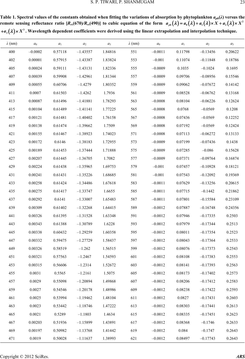

S. P. TIWARI, P. SHANMUGAM 23
Table 1. Spectral values of the constants obtained when fitting the variations of absorption by phytoplankton aph(λ) versus the
remote sensing reflectance ratio [Rrs(670)/Rrs(490)] to cubic equation of the form




2
2
XaX  

3
3
aX  
01ph
aaa  
. Wavelength dependent coefficients were derived using the linear extrapolation and interpolation technique.
λ (nm) a0 a
1 a 2 a 3 λ (nm) a0 a 1 a 2 a 3
400 –0.0002 0.57118 –1.43557 1.84816 551 –0.0011 0.11798 –0.13456 0.20622
402 0.00001 0.57915 –1.43387 1.83824 553 –0.001 0.11074 –0.11848 0.18786
405 0.00024 0.59111 –1.43131 1.82336 555 –0.0009 0.1035 –0.1024 0.1695
407 0.00039 0.59908 –1.42961 1.81344 557 –0.0009 0.09706 –0.08956 0.15546
409 0.00055 0.60706 –1.4279 1.80352 559 –0.0009 0.09062 –0.07672 0.14142
411 0.0007 0.61503 –1.4262 1.7936 561 –0.0009 0.08528 –0.06762 0.13168
413 0.00087 0.61496 –1.41881 1.78293 563 –0.0008 0.08104 –0.06226 0.12624
415 0.00104 0.61489 –1.41141 1.77225 565 –0.0008 0.0768 –0.0569 0.1208
417 0.00121 0.61481 –1.40402 1.76158 567 –0.0008 0.07436 –0.0569 0.12252
419 0.00138 0.61474 –1.39662 1.7509 569 –0.0008 0.07192 –0.0569 0.12424
421 0.00155 0.61467 –1.38923 1.74023 571 –0.0008 0.07113 –0.06272 0.13133
423 0.00172 0.6146 –1.38183 1.72955 573 –0.0009 0.07199 –0.07436 0.1438
425 0.00189 0.61453 –1.37444 1.71888 575 –0.0009 0.07285 –0.086 0.15628
427 0.00207 0.61445 –1.36705 1.7082 577 –0.0009 0.07371 –0.09764 0.16874
429 0.00224 0.61438 –1.35965 1.69753 579 –0.001 0.07457 –0.10928 0.18121
431 0.00241 0.61431 –1.35226 1.68685 581 –0.001 0.07543 –0.12092 0.19369
433 0.00258 0.61424 –1.34486 1.67618 583 –0.0011 0.07629 –0.13256 0.20615
435 0.00275 0.61417 –1.33747 1.6655 585 –0.0011 0.07715 –0.1442 0.21862
437 0.00292 0.6141 –1.33007 1.65483 587 –0.0011 0.07801 –0.15584 0.23109
439 0.00309 0.61402 –1.32268 1.64415 589 –0.0012 0.07887 –0.16748 0.24356
441 0.00326 0.61395 –1.31528 1.63348 591 –0.0012 0.07946 –0.17335 0.2503
443 0.00343 0.61388 –1.30789 1.6228 593 –0.0012 0.07979 –0.17344 0.2513
445 0.00338 0.60432 –1.29259 1.60358 595 –0.0012 0.08011 –0.17354 0.2523
447 0.00332 0.59475 –1.27729 1.58437 597 –0.0012 0.08043 –0.17364 0.2533
449 0.00326 0.58519 –1.262 1.56515 599 –0.0012 0.08076 –0.17373 0.2543
451 0.00321 0.57563 –1.2467 1.54593 601 –0.0012 0.08108 –0.17383 0.2553
453 0.00315 0.56606 –1.2314 1.52672 603 –0.0012 0.08141 –0.17393 0.2563
455 0.0031 0.5565 –1.2161 1.5075 605 –0.0012 0.08173
–0.17402 0.2573
457 0.0029 0.55098 –1.20894 1.49868 607 –0.0012 0.08206 –0.17412 0.2583
459 0.0027 0.54546 –1.20178 1.48986 609 –0.0012 0.08238 –0.17422 0.2593
461 0.0025 0.53994 –1.19462 1.48104 611 –0.0012 0.0827 –0.17431 0.2603
463 0.0023 0.53442 –1.18746 1.47222 613 –0.0012 0.08303 –0.17441 0.2613
465 0.0021 0.5289 –1.1803 1.4634 615 –0.0012 0.08335 –0.17451 0.2623
467 0.00203 0.51936 –1.15899 1.43891 617 –0.0012 0.08368 –0.1746 0.2633
469 0.00197 0.50982 –1.13768 1.41442 619 –0.0012 0.084 –0.1747 0.2643
471 0.0019 0.50028 –1.11637 1.38993 621 –0.0012 0.08497 –0.17743 0.2643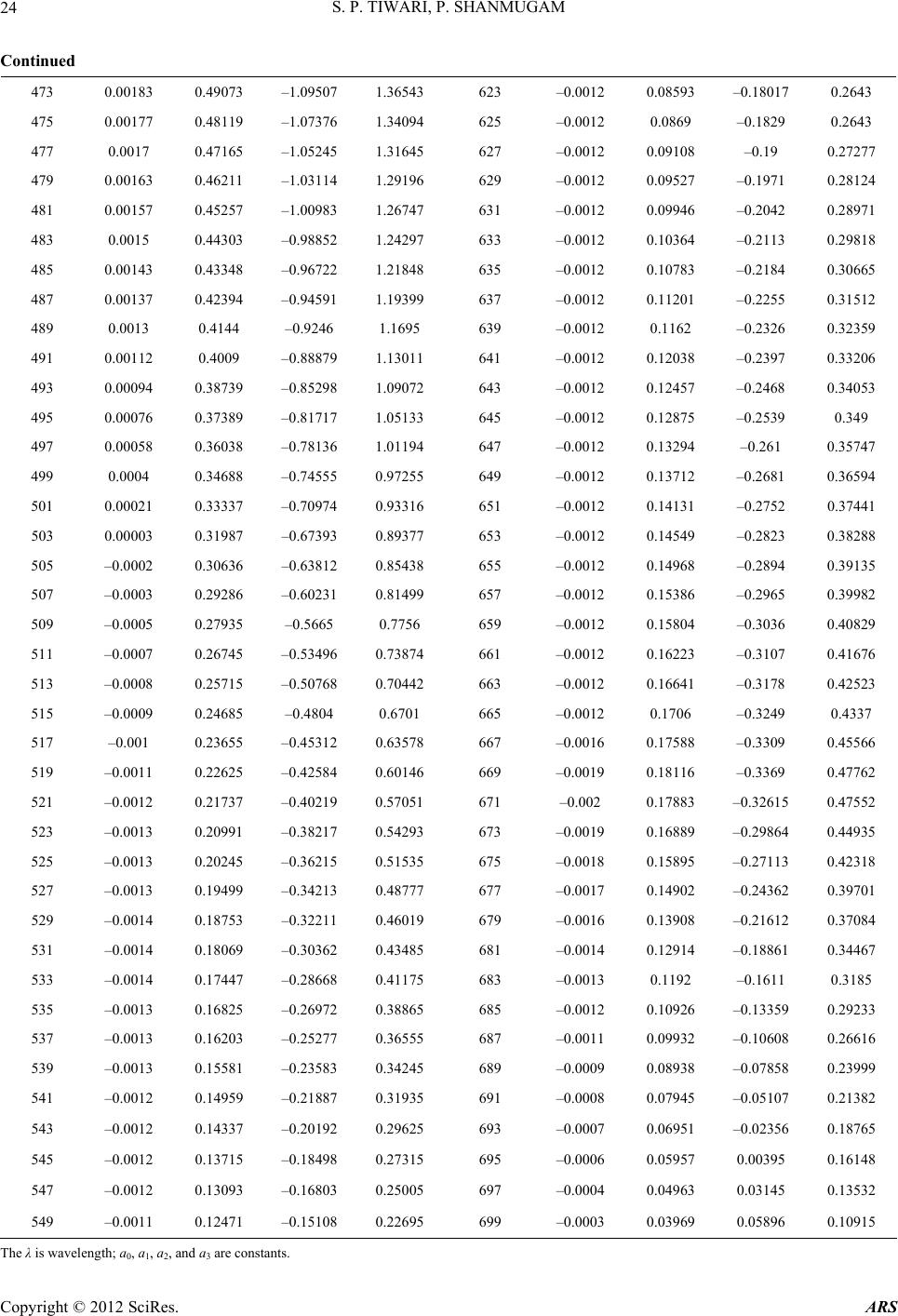

S. P. TIWARI, P. SHANMUGAM 24
Continued
473 0.00183 0.49073 –1.09507 1.36543 623 –0.0012 0.08593 –0.18017 0.2643
475 0.00177 0.48119 –1.07376 1.34094 625 –0.0012 0.0869 –0.1829 0.2643
477 0.0017 0.47165 –1.05245 1.31645 627 –0.0012 0.09108 –0.19 0.27277
479 0.00163 0.46211 –1.03114 1.29196 629 –0.0012 0.09527 –0.1971 0.28124
481 0.00157 0.45257 –1.00983 1.26747 631 –0.0012 0.09946 –0.2042 0.28971
483 0.0015 0.44303 –0.98852 1.24297 633 –0.0012 0.10364 –0.2113 0.29818
485 0.00143 0.43348 –0.96722 1.21848 635 –0.0012 0.10783 –0.2184 0.30665
487 0.00137 0.42394 –0.94591 1.19399 637 –0.0012 0.11201 –0.2255 0.31512
489 0.0013 0.4144 –0.9246 1.1695 639 –0.0012 0.1162 –0.2326 0.32359
491 0.00112 0.4009 –0.88879 1.13011 641 –0.0012 0.12038 –0.2397 0.33206
493 0.00094 0.38739 –0.85298 1.09072 643 –0.0012 0.12457 –0.2468 0.34053
495 0.00076 0.37389 –0.81717 1.05133 645 –0.0012 0.12875 –0.2539 0.349
497 0.00058 0.36038 –0.78136 1.01194 647 –0.0012 0.13294 –0.261 0.35747
499 0.0004 0.34688 –0.74555 0.97255 649 –0.0012 0.13712 –0.2681 0.36594
501 0.00021 0.33337 –0.70974
0.93316 651 –0.0012 0.14131 –0.2752 0.37441
503 0.00003 0.31987 –0.67393 0.89377 653 –0.0012 0.14549 –0.2823 0.38288
505 –0.0002 0.30636 –0.63812 0.85438 655 –0.0012 0.14968 –0.2894 0.39135
507 –0.0003 0.29286 –0.60231 0.81499 657 –0.0012 0.15386 –0.2965 0.39982
509 –0.0005 0.27935 –0.5665 0.7756 659 –0.0012 0.15804 –0.3036 0.40829
511 –0.0007 0.26745 –0.53496 0.73874 661 –0.0012 0.16223 –0.3107 0.41676
513 –0.0008 0.25715 –0.50768 0.70442 663 –0.0012 0.16641 –0.3178 0.42523
515 –0.0009 0.24685 –0.4804 0.6701 665 –0.0012 0.1706 –0.3249 0.4337
517 –0.001 0.23655 –0.45312 0.63578 667 –0.0016 0.17588 –0.3309 0.45566
519 –0.0011 0.22625 –0.42584 0.60146 669 –0.0019 0.18116 –0.3369 0.47762
521 –0.0012 0.21737 –0.40219 0.57051 671 –0.002 0.17883 –0.32615 0.47552
523 –0.0013 0.20991 –0.38217 0.54293 673 –0.0019 0.16889 –0.29864 0.44935
525 –0.0013 0.20245 –0.36215 0.51535 675 –0.0018 0.15895 –0.27113 0.42318
527 –0.0013 0.19499 –0.34213 0.48777 677 –0.0017 0.14902 –0.24362 0.39701
529 –0.0014 0.18753 –0.32211 0.46019 679 –0.0016 0.13908 –0.21612 0.37084
531 –0.0014 0.18069 –0.30362 0.43485 681 –0.0014 0.12914 –0.18861 0.34467
533 –0.0014 0.17447 –0.28668 0.41175 683 –0.0013 0.1192 –0.1611 0.3185
535 –0.0013 0.16825 –0.26972 0.38865 685 –0.0012 0.10926 –0.13359 0.29233
537 –0.0013 0.16203 –0.25277 0.36555 687 –0.0011 0.09932 –0.10608 0.26616
539 –0.0013 0.15581 –0.23583 0.34245 689 –0.0009 0.08938 –0.07858 0.23999
541 –0.0012 0.14959 –0.21887 0.31935 691 –0.0008 0.07945 –0.05107 0.21382
543 –0.0012 0.14337 –0.20192 0.29625 693 –0.0007 0.06951 –0.02356 0.18765
545 –0.0012 0.13715 –0.18498 0.27315 695 –0.0006 0.05957 0.00395 0.16148
547 –0.0012 0.13093 –0.16803 0.25005 697 –0.0004 0.04963 0.03145 0.13532
549 –0.0011 0.12471 –0.15108 0.22695 699 –0.0003 0.03969 0.05896 0.10915
The λ is wavelength; a0, a1, a2, and a3 are constants.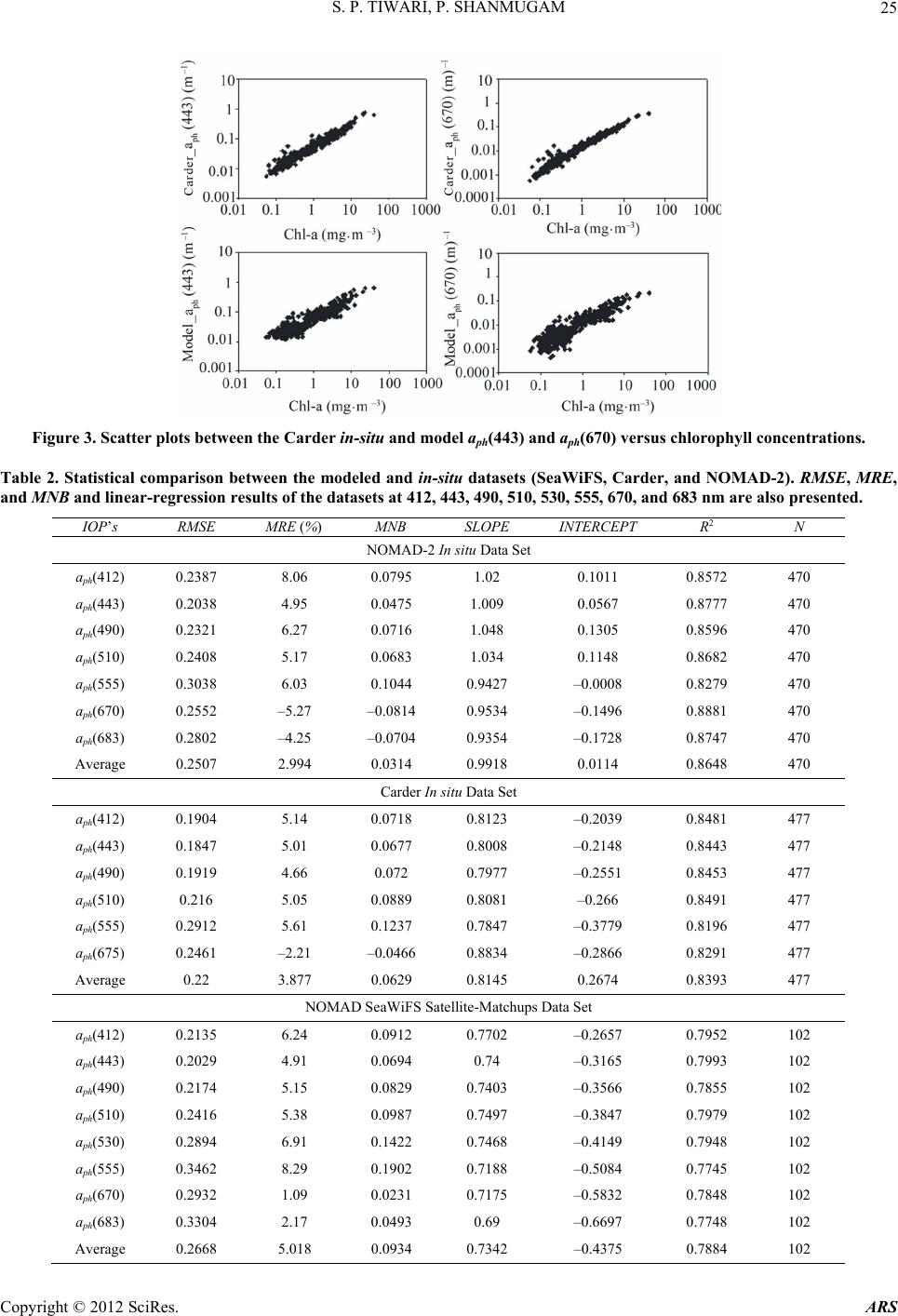

S. P. TIWARI, P. SHANMUGAM 25
Figure 3. Scatter plots between the Carder in-situ and model aph(443) and aph(670) versus chlorophyll concentrations.
Table 2. Statistical comparison between the modeled and in-situ datasets (SeaWiFS, Carder, and NOMAD-2). RMSE, MRE,
and MNB and linear-regression results of the datasets at 412, 443, 490, 510, 530, 555, 670, and 683 nm are also presented.
IOP’s RMSE MRE (%) MNB SLOPE INTERCEPT R2 N
NOMAD-2 In situ Data Set
aph(412) 0.2387 8.06 0.0795 1.02 0.1011 0.8572 470
aph(443) 0.2038 4.95 0.0475 1.009 0.0567 0.8777 470
aph(490) 0.2321 6.27 0.0716 1.048 0.1305 0.8596 470
aph(510) 0.2408 5.17 0.0683 1.034 0.1148 0.8682 470
aph(555) 0.3038 6.03 0.1044 0.9427 –0.0008 0.8279 470
aph(670) 0.2552 –5.27 –0.0814 0.9534 –0.1496 0.8881 470
aph(683) 0.2802 –4.25 –0.0704 0.9354 –0.1728 0.8747 470
Average 0.2507 2.994 0.0314 0.9918 0.0114 0.8648 470
Carder In situ Data Set
aph(412) 0.1904 5.14 0.0718 0.8123 –0.2039 0.8481 477
aph(443) 0.1847 5.01 0.0677 0.8008 –0.2148 0.8443 477
aph(490) 0.1919 4.66 0.072 0.7977 –0.2551 0.8453 477
aph(510) 0.216 5.05 0.0889 0.8081 –0.266 0.8491 477
aph(555) 0.2912 5.61 0.1237 0.7847 –0.3779 0.8196 477
aph(675) 0.2461 –2.21 –0.0466 0.8834 –0.2866 0.8291 477
Average 0.22 3.877 0.0629 0.8145 0.2674 0.8393 477
NOMAD SeaWiFS Satellite-Matchups Data Set
aph(412) 0.2135 6.24 0.0912 0.7702 –0.2657 0.7952 102
aph(443) 0.2029 4.91 0.0694 0.74 –0.3165 0.7993 102
aph(490) 0.2174 5.15 0.0829 0.7403 –0.3566 0.7855 102
aph(510) 0.2416 5.38 0.0987 0.7497 –0.3847 0.7979 102
aph(530) 0.2894 6.91 0.1422 0.7468 –0.4149 0.7948 102
aph(555) 0.3462 8.29 0.1902 0.7188 –0.5084 0.7745 102
aph(670) 0.2932 1.09 0.0231 0.7175 –0.5832 0.7848 102
aph(683) 0.3304 2.17 0.0493 0.69 –0.6697 0.7748 102
Average 0.2668 5.018 0.0934 0.7342 –0.4375 0.7884 102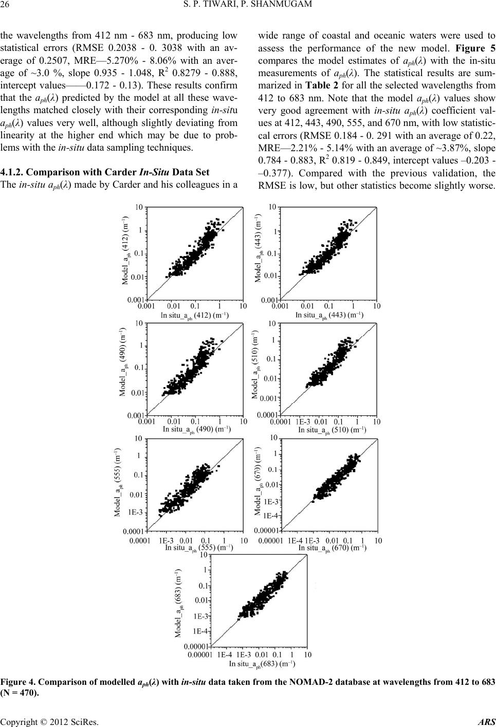

S. P. TIWARI, P. SHANMUGAM
Copyright © ARS
26
the wavelengths from 412 nm - 683 nm, producing low
statistical errors (RMSE 0.2038 - 0. 3038 with an av-
erage of 0.2507, MRE—5.270% - 8.06% with an aver-
age of ~3.0 %, slope 0.935 - 1.048, R2 0.8279 - 0.888,
intercept values——0.172 - 0.13). These results confirm
that the aph(λ) predicted by the model at all these wave-
lengths matched closely with their corresponding in-situ
aph(λ) values very well, although slightly deviating from
linearity at the higher end which may be due to prob-
lems with the in-situ data sampling techniques.
wide range of coastal and oceanic waters were used to
assess the performance of the new model. Figure 5
compares the model estimates of aph(λ) with the in-situ
measurements of aph(λ). The statistical results are sum-
marized in Table 2 for all the selected wavelengths from
412 to 683 nm. Note that the model aph(λ) values show
very good agreement with in-situ aph(λ) coefficient val-
ues at 412, 443, 490, 555, and 670 nm, with low statistic-
cal errors (RMSE 0.184 - 0. 291 with an average of 0.22,
MRE—2.21% - 5.14% with an average of ~3.87%, slope
0.784 - 0.883, R2 0.819 - 0.849, intercept values –0.203 -
–0.377). Compared with the previous validation, the
RMSE is low, but other statistics become slightly worse.
4.1.2. Comparison with Carder In-Situ Dat a Set
The in-situ aph(λ) made by Carder and his colleagues in a
Figure 4. Comparison of modelled aph(λ) with in-situ data taken from the NOMAD-2 database at wavelengths from 412 to 683
(N = 470).
2012 SciRes.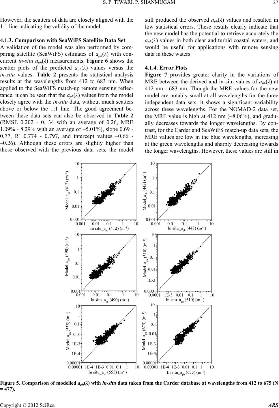

S. P. TIWARI, P. SHANMUGAM 27
However, the scatters of data are closely aligned with the
1:1 line indicating the validity of the model.
4.1.3. Comparison with SeaWiFS Satellite Data Set
A validation of the model was also performed by com-
paring satellite (SeaWiFS) estimates of aph(λ) with con-
current in-situ aph(λ) measurements. Figure 6 shows the
scatter plots of the predicted aph(λ) values versus the
in-situ values. Table 2 presents the statistical analysis
results at the wavelengths from 412 to 683 nm. When
applied to the SeaWiFS match-up remote sensing reflec-
tance, it can be seen that the aph(λ) values from the model
closely agree with the in-situ data, without much scatters
above or below the 1:1 line. The good agreement be-
tween these data sets can also be observed in Table 2
(RMSE 0.202 - 0. 34 with an average of 0.26, MRE
1.09% - 8.29% with an average of ~5.01%), slope 0.69 -
0.77, R2 0.774 - 0.797, and intercept values –0.66 -
–0.26). Although these errors are slightly higher than
those observed with the previous data sets, the model
still produced the observed aph(λ) values and resulted in
low statistical errors. These results clearly indicate that
the new model has the potential to retrieve accurately the
aph(λ) values in both clear and turbid coastal waters, and
would be useful for applications with remote sensing
data in these waters.
4.1.4. Error Plots
Figure 7 provides greater clarity in the variations of
MRE between the derived and in-situ values of aph(λ) at
412 nm - 683 nm. Though the MRE values for the new
model are notably small at all wavelengths for the three
independent data sets, it shows a significant variability
across these wavelengths. For the NOMAD-2 data set,
the MRE value is high at 412 nm (~8.06%), and gradu-
ally decreases towards the longer wavelengths. By con-
trast, for the Carder and SeaWiFS match-up data sets, the
MRE values are low in the blue wavelengths, increasing
at the green wavelengths and sharply decreasing towards
the longer wavelengths. However, these values are still in
Figure 5. Comparison of modelled aph(λ) with in-situ data taken from the Carder database at wavelengths from 412 to 675 (N
= 477).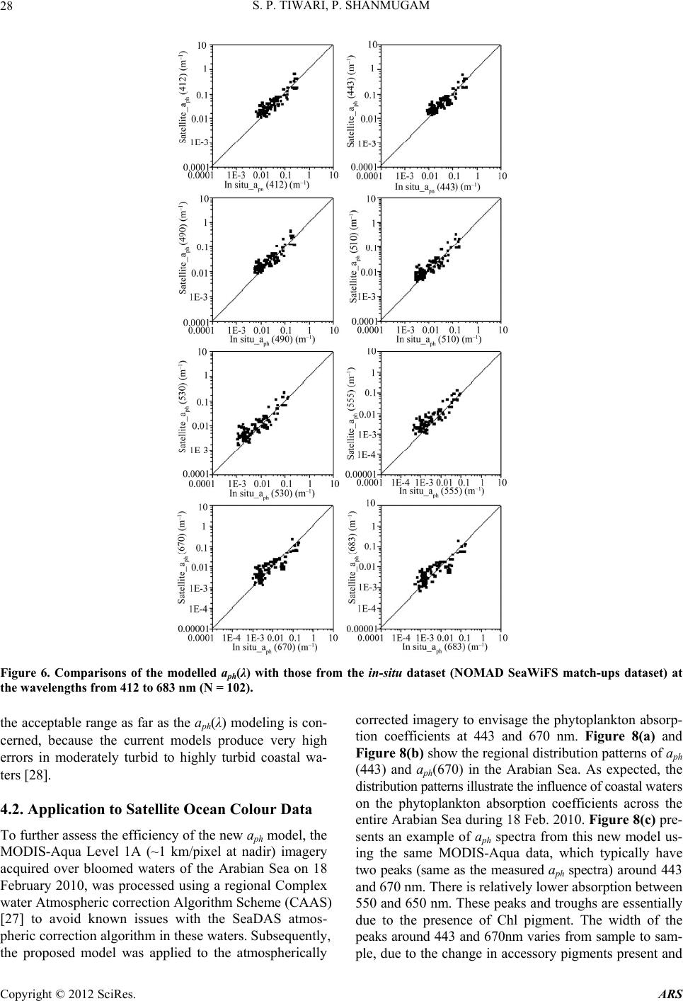

S. P. TIWARI, P. SHANMUGAM 28
Figure 6. Comparisons of the modelled aph(λ) with those from the in-situ dataset (NOMAD SeaWiFS match-ups dataset) at
the wavelengths from 412 to 683 nm (N = 102).
the acceptable range as far as the aph(λ) modeling is con-
cerned, because the current models produce very high
errors in moderately turbid to highly turbid coastal wa-
ters [28].
4.2. Application to Satellite Ocean Colour Data
To further assess the efficiency of the new aph model, the
MODIS-Aqua Level 1A (~1 km/pixel at nadir) imagery
acquired over bloomed waters of the Arabian Sea on 18
February 2010, was processed using a regional Complex
water Atmospheric correction Algorithm Scheme (CAAS)
[27] to avoid known issues with the SeaDAS atmos-
pheric correction algorithm in these waters. Subsequently,
the proposed model was applied to the atmospherically
corrected imagery to envisage the phytoplankton absorp-
tion coefficients at 443 and 670 nm. Figure 8(a) and
Figure 8(b) show the regional distribution patterns of aph
(443) and aph(670) in the Arabian Sea. As expected, the
distribution patterns illustrate the influence of coastal waters
on the phytoplankton absorption coefficients across the
entire Arabian Sea during 18 Feb. 2010. Figure 8(c) pre-
sents an example of aph spectra from this new model us-
ing the same MODIS-Aqua data, which typically have
two peaks (same as the measured aph spectra) around 443
and 670 nm. There is relatively lower absorption between
550 and 650 nm. These peaks and troughs are essentially
due to the presence of Chl pigment. The width of the
peaks around 443 and 670nm varies from sample to sam-
ple, due to the change in accessory pigments present and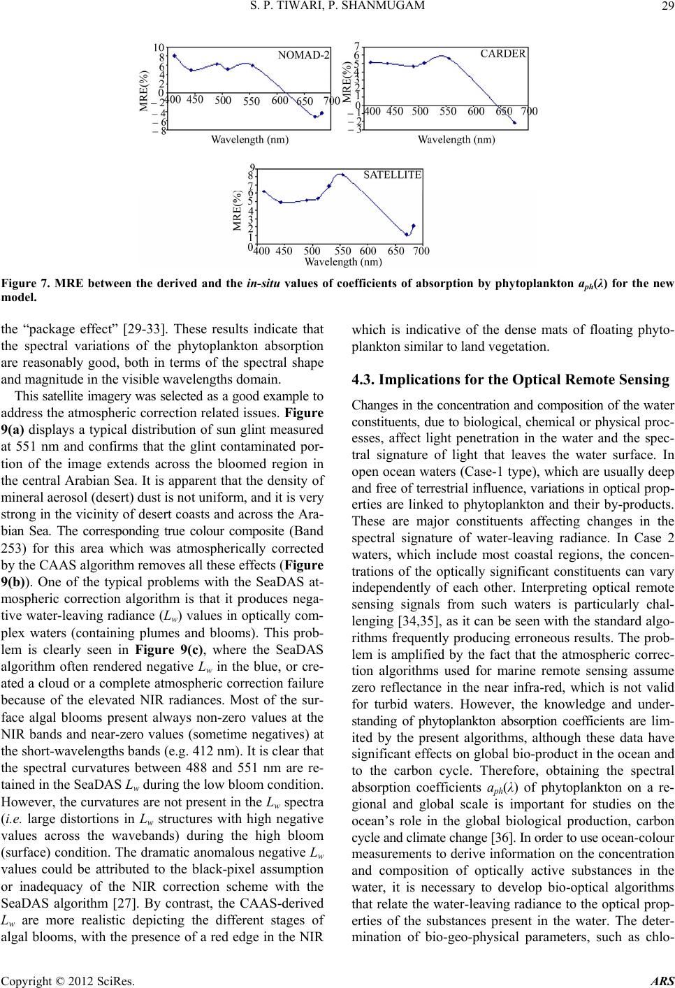

S. P. TIWARI, P. SHANMUGAM 29
Figure 7. MRE between the derived and the in-situ values of coefficients of absorption by phytoplankton aph(λ) for the new
model.
the “package effect” [29-33]. These results indicate that
the spectral variations of the phytoplankton absorption
are reasonably good, both in terms of the spectral shape
and magnitude in the visible wavelengths domain.
This satellite imagery was selected as a good example to
address the atmospheric correction related issues. Figure
9(a) displays a typical distribution of sun glint measured
at 551 nm and confirms that the glint contaminated por-
tion of the image extends across the bloomed region in
the central Arabian Sea. It is apparent that the density of
mineral aerosol (desert) dust is not uniform, and it is very
strong in the vicinity of desert coasts and across the Ara-
bian Sea. The corresponding true colour composite (Band
253) for this area which was atmospherically corrected
by the CAAS algorithm removes all these effects (Figure
9(b)). One of the typical problems with the SeaDAS at-
mospheric correction algorithm is that it produces nega-
tive water-leaving radiance (Lw) values in optically com-
plex waters (containing plumes and blooms). This prob-
lem is clearly seen in Figure 9(c), where the SeaDAS
algorithm often rendered negative Lw in the blue, or cre-
ated a cloud or a complete atmospheric correction failure
because of the elevated NIR radiances. Most of the sur-
face algal blooms present always non-zero values at the
NIR bands and near-zero values (sometime negatives) at
the short-wavelengths bands (e.g. 412 nm). It is clear that
the spectral curvatures between 488 and 551 nm are re-
tained in the SeaDAS Lw during the low bloom condition.
However, the curvatures are not present in the Lw spectra
(i.e. large distortions in Lw structures with high negative
values across the wavebands) during the high bloom
(surface) condition. The dramatic anomalous negative Lw
values could be attributed to the black-pixel assumption
or inadequacy of the NIR correction scheme with the
SeaDAS algorithm [27]. By contrast, the CAAS-derived
Lw are more realistic depicting the different stages of
algal blooms, with the presence of a red edge in the NIR
which is indicative of the dense mats of floating phyto-
plankton similar to land vegetation.
4.3. Implications for the Optical Remote Sensing
Changes in the concentration and composition of the water
constituents, due to biological, chemical or physical proc-
esses, affect light penetration in the water and the spec-
tral signature of light that leaves the water surface. In
open ocean waters (Case-1 type), which are usually deep
and free of terrestrial influence, variations in optical prop-
erties are linked to phytoplankton and their by-products.
These are major constituents affecting changes in the
spectral signature of water-leaving radiance. In Case 2
waters, which include most coastal regions, the concen-
trations of the optically significant constituents can vary
independently of each other. Interpreting optical remote
sensing signals from such waters is particularly chal-
lenging [34,35], as it can be seen with the standard algo-
rithms frequently producing erroneous results. The prob-
lem is amplified by the fact that the atmospheric correc-
tion algorithms used for marine remote sensing assume
zero reflectance in the near infra-red, which is not valid
for turbid waters. However, the knowledge and under-
standing of phytoplankton absorption coefficients are lim-
ited by the present algorithms, although these data have
significant effects on global bio-product in the ocean and
to the carbon cycle. Therefore, obtaining the spectral
absorption coefficients aph(λ) of phytoplankton on a re-
gional and global scale is important for studies on the
ocean’s role in the global biological production, carbon
cycle and climate change [36]. In order to use ocean-colour
measurements to derive information on the concentration
and composition of optically active substances in the
water, it is necessary to develop bio-optical algorithms
that relate the water-leaving radiance to the optical prop-
erties of the substances present in the water. The deter-
mination of bio-geo-physica parameters, such as chlo- l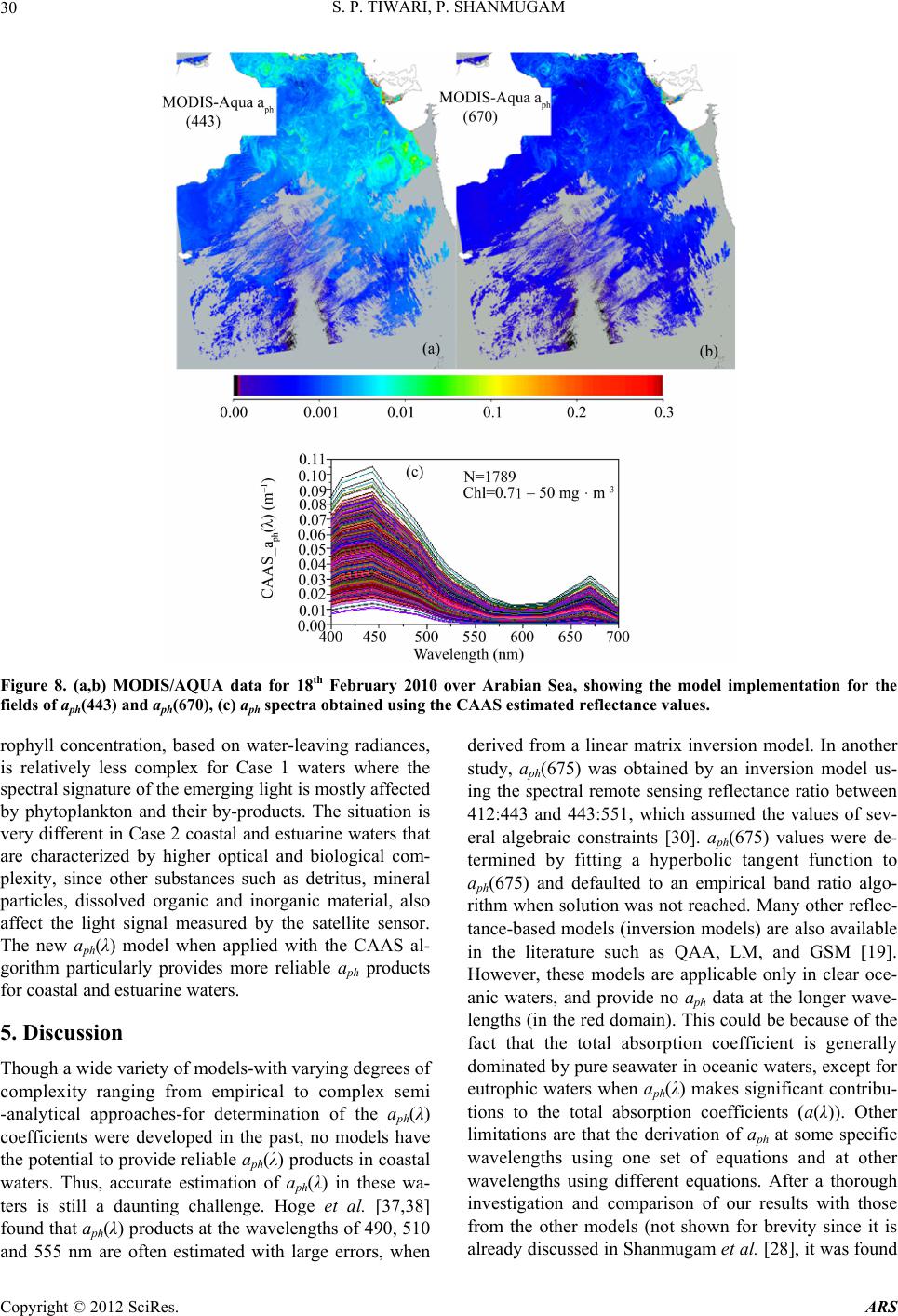

S. P. TIWARI, P. SHANMUGAM 30
Figure 8. (a,b) MODIS/AQUA data for 18th February 2010 over Arabian Sea, showing the model implementation for the
fields of aph(443) and aph(670), (c) aph spectra obtained using the CAAS estimated reflectance values.
rophyll concentration, based on water-leaving radiances,
is relatively less complex for Case 1 waters where the
spectral signature of the emerging light is mostly affected
by phytoplankton and their by-products. The situation is
very different in Case 2 coastal and estuarine waters that
are characterized by higher optical and biological com-
plexity, since other substances such as detritus, mineral
particles, dissolved organic and inorganic material, also
affect the light signal measured by the satellite sensor.
The new aph(λ) model when applied with the CAAS al-
gorithm particularly provides more reliable aph products
for coastal and estuarine waters.
5. Discussion
Though a wide variety of models-with varying degrees of
complexity ranging from empirical to complex semi
-analytical approaches-for determination of the aph(λ)
coefficients were developed in the past, no models have
the potential to provide reliable aph(λ) products in coastal
waters. Thus, accurate estimation of aph(λ) in these wa-
ters is still a daunting challenge. Hoge et al. [37,38]
found that aph(λ) products at the wavelengths of 490, 510
and 555 nm are often estimated with large errors, when
derived from a linear matrix inversion model. In another
study, aph(675) was obtained by an inversion model us-
ing the spectral remote sensing reflectance ratio between
412:443 and 443:551, which assumed the values of sev-
eral algebraic constraints [30]. aph(675) values were de-
termined by fitting a hyperbolic tangent function to
aph(675) and defaulted to an empirical band ratio algo-
rithm when solution was not reached. Many other reflec-
tance-based models (inversion models) are also available
in the literature such as QAA, LM, and GSM [19].
However, these models are applicable only in clear oce-
anic waters, and provide no aph data at the longer wave-
lengths (in the red domain). This could be because of the
fact that the total absorption coefficient is generally
dominated by pure seawater in oceanic waters, except for
eutrophic waters when aph(λ) makes significant contribu-
tions to the total absorption coefficients (a(λ)). Other
limitations are that the derivation of aph at some specific
wavelengths using one set of equations and at other
wavelengths using different equations. After a thorough
investigation and comparison of our results with those
from the other models (not shown for brevity since it is
already discussed in Shanmugam et al. [28], it was found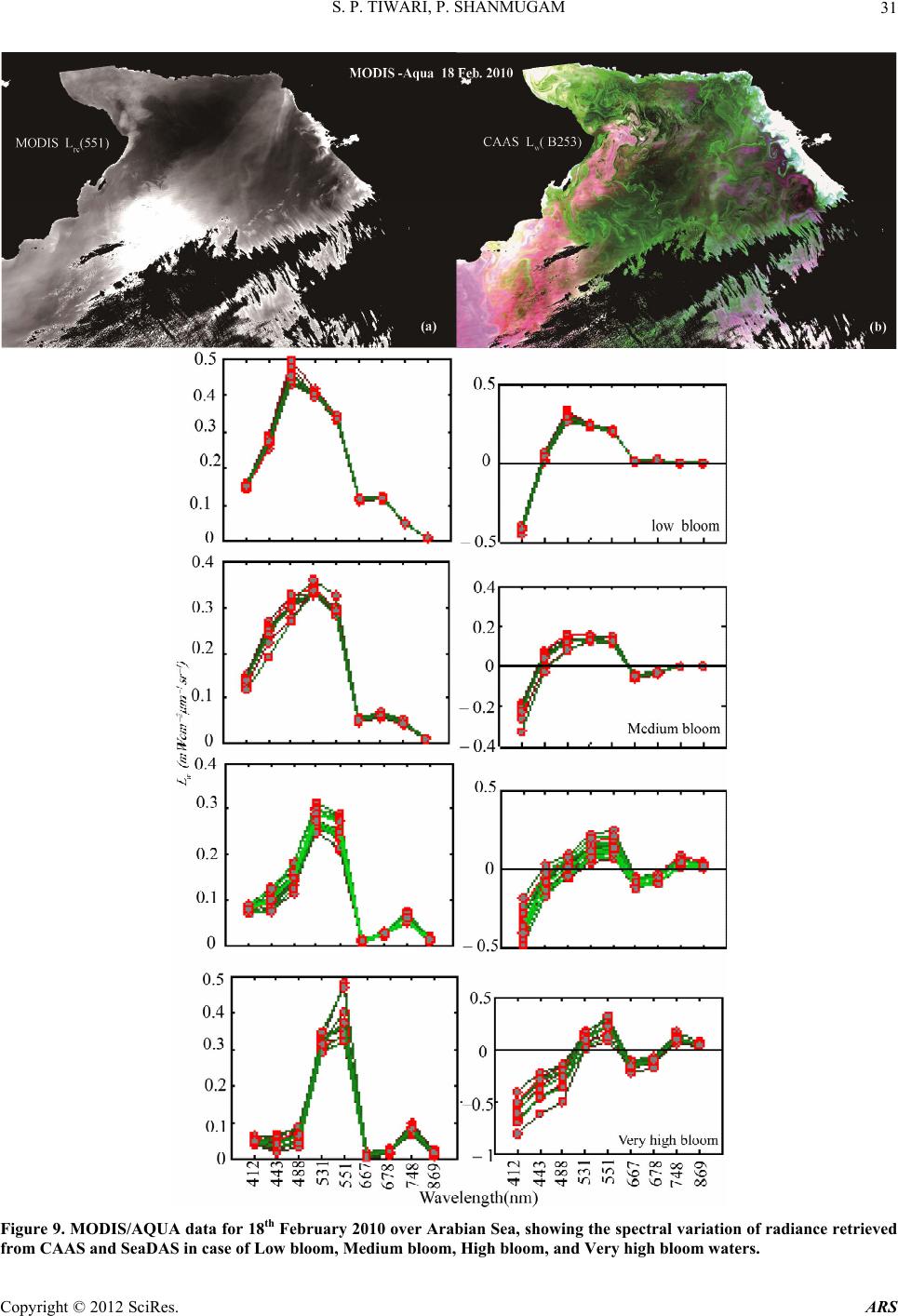

S. P. TIWARI, P. SHANMUGAM 31
Figure 9. MODIS/AQUA data for 18th February 2010 over Arabian Sea, showing the spectral variation of radiance retrieved
from CAAS and SeaDAS in case of Low bloom, Medium bloom, High bloom, and Ve ry high bloom w a ters.

S. P. TIWARI, P. SHANMUGAM 32
that the new model is inherently more flexible for deter-
mination of aph coefficients at any wavelengths in the
visible domain.
6. Conclusion
The new model has significant advantages over other
models, since it relies on the Rrs(670) /Rrs(490) ratio
which is not significantly influenced by materials other
than phytoplankton. Validation of the model with inde-
pendent in-situ data sets gave encouraging results. The
model-predicted aph(λ) values were found to be in good
agreement with in-situ data from coastal/oceanic waters.
The model wavelengths of the SeaWiFS sensor (412 to
683 nm). Though the errors were low (e.g., MRE 8%),
scatter plots showed slight differences between the model
and in-situ aph(λ) values. The difference may arise due to
several reasons; for instance, Rrs(λ) measurements made
with different instruments with different calibration and
correction procedures as well as environmental conditions.
It was demonstrated that the atmospheric correction of
satellite ocean colour data could introduce very high errors
in complex waters. However, such problems could be
eliminated when the water-leaving radiance signals are
estimated with the CAAS algorithm. Thus, the aph(λ)
model may be applied along with the CAAS algorithm,
in order to retrieve more reliable aph(λ) values in opti-
cally complex waters. A MODIS-Aqua example showed
striking features of the distribution pattern of phyto-
plankton absorption coefficients in bloomed waters in the
Arabian Sea. In conclusion, this is the first study to esti-
mate aph(λ) values at all the visible wavelengths. Thus, it
provides new opportunities for improving the phyto-
plankton inversion modelling based on the coefficients as
given in Table 1. Our future effort will include addi-
tional validation and tests based on more in-situ and sat-
ellite data, and refining the model coefficients in order to
provide more accurate phytoplankton absorption coef-
ficients in complex waters.
7. Acknowledgements
This work was supported by INCOIS under the grant
(OEC/1011/102/INCO/PSHA) of the SATCORE pro-
gram. The authors would like to thank the NASA Ocean
Biology Processing Group for making available the
global, high quality bio-optical (NOMAD) data set and
the LAC MODIS-Aqua to this study. The authors would
like to thank J. P. Cannizzaro and C. Hu for providing
the bio-optical datasets of Prof. K. L. Carder.
REFERENCES
[1] A. Morel and L. Prieur, “Analysis of Variations in Ocean
Colour,” Limnology and Oceanography, Vol. 22, No. 4,
1977, pp. 709-722. doi:10.4319/lo.1977.22.4.0709
[2] A. Morel and S. Maritorena, “Bio-Optical Properties of
Oceanic Waters: A Reappraisal,” Journal of Geophysical
research, Vol. 106, No. C4, 2001, pp. 7163-7180.
doi:10.1029/2000JC000319
[3] H. R. Gordon, O. B. Brown, R. H. Evans, J. W. Brown, R.
C. Smith, K. S. Baker and D. K. Clark, “A Semi-Analytic
Model of Ocean Colour,” Journal of Geophysical Re-
search, Vol. 9, No. D9, 1988, pp. 10909-10924.
doi:10.1029/JD093iD09p10909
[4] A. Morel, “Optical Modeling of the Upper Ocean in Rela-
tion to Its Biogenous Matter Content (Case I Waters),”
Journal of Geophysical Research, Vol. 93, No. C9, 1988,
pp. 10749-10768. doi:10.1029/JC093iC09p10749
[5] T. Platt and S. Sathyendranath, “Oceanic Primary Pro-
duction: Estimation by Remote Sensing at Local and Re-
gional Scales,” Science, Vol. 241, No. 4873, 1988, pp.
1613-1620. doi:10.1126/science.241.4873.1613
[6] H. M. Sosik and B. G. Mitchell, “Light Absorption by
Phytoplankton, Photosynthetic Pigments and Detritus in
the California Current System,” Deep Sea-Research, Vol.
42, No. 10, 1995, pp. 1717-1748.
doi:10.1016/0967-0637(95)00081-G
[7] E. H. S. Van Duin, G. Blom, F. J. Los, R. Maffione, R.
Zimmerman, C. F. Cerco, D. Mark, E. P. H. Best, Van
Duin, et al., “Modeling Underwater Light Climate in Re-
lation to Sedimentation, Resuspension, Water Quality and
Autotrophic Growth,” Hydrobiologia, Vol. 444, No. 1-3,
2001, pp. 25-42. doi:10.1023/A:1017512614680
[8] A. Morel, B. Gentili, M. Chami and J. Ras, “Bio-Optical
Properties of High Chlorophyll Case 1 Waters, and of
Yellow-Substance-Dominated Case 2 Waters,” Deep-Sea
Research Part I, Vol. 53, No. 9, 2006, pp. 1439-1559.
doi:10.1016/j.dsr.2006.07.007
[9] N. Hoepffner and S. Sathyendranath, “Determination of
the Major Groups of Phytoplankton Pigments from the
Absorption Spectra of Total Particulate Matter,” Journal
of Geophysical Research, Vol. 98, No. C12, 1993, pp.
22789-22804. doi:10.1029/93JC01273
[10] A. Ciotti, M. R. Lewis and J. J. Cullen, “Assessment of
the Relationship between Dominant Cell Size in Natural
Phytoplakton Communities and the Spectral Shape of the
Absorption Coefficient,” Limnology and Oceanography,
Vol. 47, No. 2, 2002, pp. 404-417.
doi:10.4319/lo.2002.47.2.0404
[11] J. R. Moisan, T. A. H. Moisan and M. A. Linkswiler, “An
Inverse Modeling Approach to Estimating Phytoplankton
Pigment Concentrations from Phytoplankton Absorption
Spectra,” Journal of Geophysical Research, Vol. 116, No.
C09018, 2011.
[12] L. Prieur and S. Sathyendranath, “An Optical Classifica-
tion of Coastal and Oceanic Waters Based on the Specific
Spectral Absorption Curves of Phytoplankton Pigments,
Dissolved Organic Matter, and Other Particulate Materi-
als,” Limnology and Oceanography, Vol. 26, No. 4, 1981,
pp. 671-689. doi:10.4319/lo.1981.26.4.0671
[13] E. Millan-Nunez, M. E. Sieracki, R. Millan-Nunez, J. R.

S. P. TIWARI, P. SHANMUGAM 33
Lara-Lara, G. Gaxiola-Castro and C. C. Trees, “Specific
Absorption Coefficient and Phytoplankton Biomass in the
Southern Region of the California Current,” Deep Sea
Research, Part II, Vol. 51, No. 6-9, 2004, pp. 817-826.
doi:10.1016/j.dsr2.2004.05.023
[14] S. A. Garver and D. Siegel, “Inherent Optical Property
Inversion of Ocean Colour Spectra and Its Biogeochemi-
cal Interpretation 1. Time Series from the Sargasso Sea,”
Journal of Geophysical Research, Vol. 102, No. C8, 1997,
pp. 18607-18625. doi:10.1029/96JC03243
[15] S. Maritorena, D. A. Siegel and A. R. Peterson, “Optimi-
zation of a Semianalytical Ocean Colour Model for
Global-Scale Applications,” Applied Optics, Vol. 41, No.
15, 2002, pp. 2705-2714. doi:10.1364/AO.41.002705
[16] Z. P. Lee, K. L. Carder and R. Arnone, “Deriving Inher-
ent Optical Roperties from Water Colour: A Multi-Band
Quasi-Analytical Algorithm or Optically Deep Waters,”
Applied Optics, Vol. 41, No. 27, 2002, pp. 5755-5772.
doi:10.1364/AO.41.005755
[17] P. Shanmugam, Y. H. Ahn, J. H. Ryu and B. Sundara-
balan, “An Evaluation of Inversion Models for Retrieval
of Inherent Optical Properties from Ocean Colour in
Coastal and Open Sea Waters around Korea,” Journal of
Oceanography, Vol. 66, No. 6, 2010, pp. 815-830.
doi:10.1007/s10872-010-0066-0
[18] T. J. Smyth, G. F. Moore, T. Hirata and J. Aiken, “Se-
mianalytical Model for the Derivation of Ocean Colour
Inherent Optical Properties: Description, Implementation,
and Performance Assessment,” Applied Optics, Vol. 45,
No. 31, 2006, pp. 8116-8131.
doi:10.1364/AO.45.008116
[19] E. Boss and C. Roesler, “Over Constrained Linear Matrix
Inversion with Tatistical Selection,” In: Z. Lee, Ed., Re-
mote Sensing of Inherent Optical Properties: Fundamen-
tals, Tests of Algorithms, and Applications, IOCCG,
Dartmouth, NS, Canada, IOCCG Rep. 5, 2006.
[20] H. C. van de Hulst, “Light Scattering by Small Particles,”
Dover, Mineola, 1981, 470 p.
[21] R. W. Preisendorfer, “Application of Radiative Transfer
theory to Light Measurements in the Sea,” Union of Geo-
detic Geophysical Institute Monograph, Vol. 10, 1961, pp.
11-30.
[22] M. Pope and E. S. Fry, “Absorption Spectrum (380 - 700
nm) of Pure Water. II. Integrating Cavity Measurements,”
Applied Optics, Vol. 36, No. 33, 1997, pp. 8710-8723.
doi:10.1364/AO.36.008710
[23] R. C. Smith and K. S. Baker, “Optical Properties of the
Clearest Natural Waters,” Applied Optics, Vol. 20, No. 2,
1981, pp. 177-184. doi:10.1364/AO.20.000177
[24] A. Bricaud, A. Morel and L. Prieur, “A Absorption by
Dissolved Organic Matter in the Sea (yellow substance)
the UV and Visible Domains,” Limnology and Oceano-
graphy, Vol. 26, No. 1, 1981, pp. 43-53.
doi:10.4319/lo.1981.26.1.0043
[25] A. Bricaud, M. Babin, A. Morel and H. Claustre,
“Variability in the Chlorophyll-Specific Absorption Co-
efficients of Natural Phytoplankton: Analysis and Para-
meterization,” Journal of Geophysical Research, Vol. 100,
No. C7, 1995, pp. 13321-13332.
doi:10.1029/95JC00463
[26] A. Bricaud, A. Morel, M. Babin, K. Allali and H.
Claustre, “Variations of Light Absorption by Suspended
Particles with Chlorophyll a Concentration in Oceanic
(Case 1) Waters: Analysis and Implications for Bio-
Optical Models,” Journal of Geophysical Research, Vol.
103, No. C13, 1998, pp. 31033-31044.
doi:10.1029/98JC02712
[27] P. Shanmugam, “CAAS: An Atmospheric Correction
Algorithm for the Remote Sensing of Complex Waters,”
Annales Geophysicae, Vol. 30, No. 1, 2012, pp. 203-220.
doi:10.5194/angeo-30-203-2012
[28] P. Shanmugam, Y. H. Ahn, J. H. Ryu and B. Sundara-
balan, “An Evaluation of Inversion Models for Retrieval
of Inherent Optical Properties from Ocean Colour in
Coastal and Open Sea around Korea,” Journal of Ocean-
ography, Vol. 66, 2010, pp. 815-830.
doi:10.1007/s10872-010-0066-0
[29] K. L. Carder, S. K. Hawes, K. A. Baker, R. C. Smith, R.
G. Steward and B. G. Mitchell, “Reflectance Model for
Quantifying Chlorophyll a in the Presence of Productivity
Degradation Products,” Journal of Geophysical Research ,
Vol. 96, No. C11, 1991, pp. 599-611.
doi:10.1029/91JC02117
[30] K. L. Carder, F. R. Chen, Z. P. Lee, S. K. Hawes and D.
Kamykowski, “Semianalytic Moderate-Resolution Imag-
ing Spectrometer Algorithms for Chlorophyll-a and
Absorption with Bio-Optical Domains Based on Nitrate
Depletion Temperatures,” Journal of Geophysical Re-
search, Vol. 104, No. C3, 1999, pp. 5403-5421.
doi:10.1029/1998JC900082
[31] C. S. Yentsch and D. A. Phinney, “Spectral Fluorescence:
An Ataaxonomic Tool for Studying the Structure of
Phytoplankton Populations,” Journal of Plankton Re-
search, Vol. 7, No. 5, 1985, pp. 617-632.
doi:10.1093/plankt/7.5.617
[32] C. S. Yentsch and D. A. Phinney, “A Bridge between
Ocean Optics and Microbial Ecology,” Limnology and
Oceanography, Vol. 34, No. 8, 1989, pp. 1694-l705.
doi:10.4319/lo.1989.34.8.1694
[33] J. E. O'Reilly, S. Moritorena, B. G. Mitchell, D. S. Seigel,
K. L. Carder, S. A. Garver, et al., “Ocean Colour Chloro-
phyll Algorithms for SeaWiFS,” Journal of Geophysical
Research, Vol. 103, No. C11, 1998, pp. 937-953.
[34] R. Miller, C. Del-Castillo and B. McKee, “Remote Sens-
ing of Coastal Aquatic Environments,” Springer, Dord-
recht, 2005, p. 347. doi:10.1007/978-1-4020-3100-7
[35] S. Sathyendranath, Ed., “Remote Sensing of Ocean Col-
our in Coastal, and Other Optically Complex Waters,”
Reports of the International Ocean-Colour Coordinating
Group, IOCCG, Dartmouth, NS, Canada, Rep. 3, 2000, p.
140.
[36] M. Tzortziou, A. Subramaniam, J. R. Herman, C. L.
Gallegos, P. J. Neale and H. L. W. Jr., “Remote Sensing
Reflectance and Inherent Optical Properties in the Mid
Chesapeake Bay,” Estuarine, Coastal and Shelf Science,
Vol. 72, No. 1-2, 2007, pp. 16-32.
doi:10.1016/j.ecss.2006.09.018
[37] F. E Hoge and P. E. Lyon, “Satellite Retrieval of Inherent

S. P. TIWARI, P. SHANMUGAM 34
Optical Properties by Linear Matrix Inversion of Oceanic
Radiance Models: An Analysis of Model and Radiance
Measurements,” Journal of Geophysical Research, Vol.
101, No. C7, 1996, pp. 16631-16648.
doi:10.1029/96JC01414
[38] F. E. Hoge and P. E. Lyon, “Spectral Parameters of In-
herent Optical Property Models: Method for Satellite Re-
trieval by Matrix Inversion of an Oceanic Radiance Mod-
el,” Applied Optics, Vol. 38, No. 9, 1999, pp. 1657-1662.
doi:10.1364/AO.38.001657