Paper Menu >>
Journal Menu >>
 Engineering, 2010, 2, 485-495 doi:10.4236/eng.2010.27064 Published Online July 2010 (http://www.SciRP.org/journal/eng) Copyright © 2010 SciRes. ENG 485 Dynamic Stress Intensity Factors for Three Parallel Cracks in an Infinite Plate Subject to Harmonic Stress Waves Shouetsu Itou Department of Mechanical Engineering, Kanagawa University, Yokohama, Japan E-mail: itous001@kanagawa-u.ac.jp Received February 25, 2010; revised April 9, 2010; accepted April 22, 2010 Abstract Dynamic stresses around three parallel cracks in an infinite elastic plate that is subjected to incident time-harmonic stress waves normal to the cracks have been solved. Using the Fourier transform technique, the boundary conditions are reduced to six simultaneous integral equations. To solve these equations, the differences of displacements inside the cracks are expanded in a series. The unknown coefficients in those series are solved using the Schmidt method such that the conditions inside the cracks are satisfied. Numerical calculations are carried out for some crack configurations. Keywords: Three Cracks, Time-Harmonic Problem, Stress Intensity Factor, Integral Equation, The Schmidt Method 1. Introduction A time-harmonic solution for stresses around a crack in an infinite plate was reported by Loeber and Sih [1]. In their study, they obtained the Mode III dynamic stress intensity factor during the passage of a time-harmonic anti-plane shear wave. Subsequently, they also solved the crack problem for a compression wave and a vertically polarized shear wave [2]. Adopting a somewhat different approach, the same problem was studied independently by Mal [3]. The corresponding three-dimensional solu- tions for a penny-shaped crack have been obtained by Sih and Loeber [4,5] and by Mal [6]. Materials are generally weakened by some cracks. Therefore, it is of interest to reveal the mutual effect of the cracks on the dynamic stress intensity factors. Itou solved the dynamic stresses around two collinear cracks in which a self-equilibrated system of pressure is varied harmonically with time [7]. Later, the Mode III solution was given for two collinear cracks by Itou [8]. As for three collinear cracks, Mode I solution s were determined under the condition that time-harmonic normal traction is applied to the surfaces of the cracks [9]. Materials are occasionally weakened by some parallel cracks. Takakuda solved the time-harmonic problem for two parallel cracks in an infinite plane subjected to waves that impinge perpendicular to the cracks [10]. So and Huang analyzed the Mode III stress intensity factor around two cracks located in arbitrary positions in an infinite medium subjected to incident SH waves [11]. Meguid and Wang cleared the effect of the existence of an arbitrarily located and oriented micro defect on the dynamic stress intensity factors for a finite main crack subjected to a plane incident wave [12]. Ayatollahi and Fariborz provided the analysis of multiple curved cracks in an infinite plane under in-plane time harmonic loads [13]. Itou and Haliding assumed that two small collinear cracks are situated symmetrically above a main crack in an infinite plate and provided the dynamic stress inten- sity factors dur ing passage of time-harmonic wave s [1 4 ] . A peak value of the dynamic stress intensity factor for collinear cracks in an infinite elastic plate is generally about 1.20-1.60 times larger than that of the corresponding static v alue peak i K s tatic i K. However, in the paper [10], it was found that a peak value of the dynamic stress intensity factor for two parallel cracks is significantly larger than those for the collinear cracks. For example, for an infinite plate containing two parallel cracks of length separated by a distance , the 2ahpeak i K s tatic i K ratio is 4.16 for 1.0ha [10]. It was also shown that similar results appear for two parallel cracks in an infinite orthotropic plate subjected to incident time-harmonic stress waves [15]. From this fact, it is expected that p eak static ii KK ratio will be very large for three parallel cracks during passage of the time harmonic stress waves. 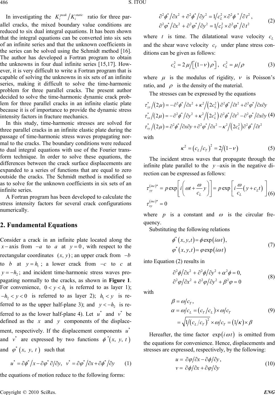 S. ITOU 486 In investigating the p eak static ii KK ratio for three par- allel cracks, the mixed boundary value conditions are reduced to six dual integral equations. It has been shown that the integral equations can be converted into six sets of an infinite series and that the unknown coefficients in the series can be solved using the Schmidt method [16]. The author has developed a Fortran program to obtain the unknowns in four dual infinite series [15,17]. How- ever, it is very difficult to write a Fortran program that is capable of solvin g the unknown s in six sets of an infinite series, making it difficult to solve the time-harmonic problem for three parallel cracks. The present author decided to solve the time-harmonic dynamic crack prob- lem for three parallel cracks in an infinite elastic plate because it is of importance to provide the dynamic stress intensity factors in fracture mechanics. In this study, time-harmonic stresses are solved for three parallel cracks in an infinite elastic plate during the passage of time-harmonic stress waves propagating nor- mal to the cracks. The boundary co nditions were redu ced to dual integral equations with use of the Fourier trans- form technique. In order to solve these equations, the differences between the crack surface displacements are expanded to a series of functions that are equal to zero outside the cracks. The Schmidt method is modified so as to solve for the unknown coefficients in six sets of an infinite series. A Fortran progr am has been developed to calculate the stress intensity factors for several crack configurations numerically. 2. Fundamental Equations Consider a crack in an infinite plate located along the x axis from to at , with respect to the rectangular coordinates aa0y )(, x y; an upper crack from b to at ; a lower crack from to at ; and incident time-harmonic stress waves pro- pagating normally to the cracks, as shown in Figure 1. For convenience, is referred to as layer 1); is referred to as layer 2); is re- ferred to as the upper half-plane 3); and is re- ferred to as the lower half-plane 4). Let and be defined as the b y 2 1 hy 0 c 1 h y * u c h * v 2 h hy 1 h0y y 2 x and components of the displace- ment, respectively. If the displacement components and are expressed by two functions y * u * v *,, x yt and ,, * x yt such that ** **** ,uxyv x y (1) the equations of motion reduce to the following forms: 2*22*222 *2 2*2 2*222*2 1, 1 L T x yc t x yc t (2) where is time. The dilatational wave velocity t L c and the shear wave velocity under plane stress con- ditions can be given as follows: T c 2 21 , L c2 L c (3) where is the modulus of rigidity, is Poisson’s ratio, and is the density of the material. The stresses can be expressed by the equations *2*2222*22* *2*2222*22* *2*2*2222* 22 22 22 yy L xx L xyL 2 x ct yct xy xy x yxct (4) with 2 221 LT cc (5) The incident stress waves that propagate through the infinite plate parallel to the –axis in the negative di- rection can be expressed as follows: y * * exp exp 0 inc yy L LL inc xy pitypiyct cc (6) where is a constant and p is the circular fre- quency. Substituting the following relations * * ,, exp , ,, exp x yti t x yti t (7) into Equation (2) results in 22222 22222 0, 0 xy xy (8) with 2 , 11 T LTLT LT T c ccc c cc c (9) Hereafter, the time factor exp it is omitted from the equations for convenience. Hence, displacements and stresses are expressed, respectively, by the following: ,ux vx y y (10) Copyright © 2010 SciRes. ENG 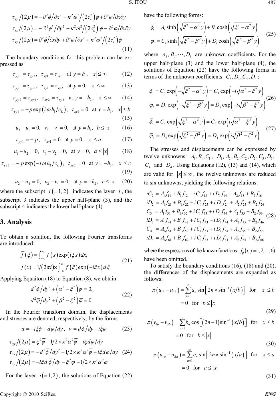 S. ITOU487 22222 2 2*22 222 222222 22 22 22 yy L xx L xy L x cxy y cx xy xc y (11) The boundary conditions for this problem can be ex- pressed as 1313 1 ,at, yyyy xyxyyh x (12) 1212 ,at0, yyyy xy xyyx (13) 2424 2 ,at, yyyy xyxyyhx (14) 1111 exp,0 at, yyL xy pihc yhx b (15) 31 311 0,0, at,uu vvyhbx (16) 11 ,0at0, yy xy py xa (17) 12 12 0,0, at0,uuvvy ax (18) 2222 exp,0at, yyL xy pihc yhx c (19) 24 242 0,0, at,uuvvy hcx (20) where the subscript indicates the layer , the subscript 3 indicates the upper half-plane (3), and the subscript 4 indicates the lower half-plane (4). 1, 2i i 3. Analysis To obtain a solution, the following Fourier transforms are introduced: exp , ()1 2exp ffxixdx f xif ix d (21) Applying Equ aiton (18) to Equation (8), we obtain : 2222 2222 0, 0 ddy ddy (22) In the Fourier transform domain, the displacements and stresses are denoted, respectively, by the forms ,ui ddyvddyi (23) 222 22 22 222 212 212 212 yy xx xy id dy ddy idd id dy y (24) For the layer , the solutions of Equation (22) have the following forms: 1, 2i 22 22 22 22 sinh cosh sinh cosh ii i ii i A yB y CyD y (25) where ,,, ii i A BD are unknown coefficients. For the upper half-plane (3) and the lower half-plane (4), the solutions of Equation (22) have the following forms in terms of the unknown coefficients : 3344 ,,,CDCD 22 22 33 3 22 22 33 3 exp exp exp exp CyCi DyDi y y (26) 22 22 44 4 22 22 44 4 exp exp exp exp CyCi DyDi y y (27) The stresses and displacements can be expressed by twelve unknowns: 111 ,, A BC, and . Using Equations (12), (13) and (14), which are valid for 1222233 ,,,,,,,DABCDCD 4 C4 D x , the twelve unknowns are reduced to six unknowns, yielding the following relations: 21 111 121 131142 15216 21 211 221 23124225226 31 311 321 331342 35236 31 411 421 431 44245246 41511 521 531542 552 iCAfBfiCfi DfAfBf iDAfBfiCfiDfAfBf CAfBfiCfiDfAfBf iDAfBfiCfi DfAfBf CAfBfiCfiDfAfB 56 41 611621 631 64265266 f iDAfBfiCfi DfAfBf (28) where the expressions of the known functions ,1,2,,6 ij fij have been omitted. To satisfy the boundary conditions (16), (18) and (20), the differences of the displacements are expanded as follows: 1 13 1sin 2sinfor 0for bb n n uuanxbxb bx (29) 1 13 1cos21sinfor 0for bb n n vv bnxbxb bx (30) 1 12 1sin 2sinfor 0for aa n n uuc nxaxa ax (31) Copyright © 2010 SciRes. ENG 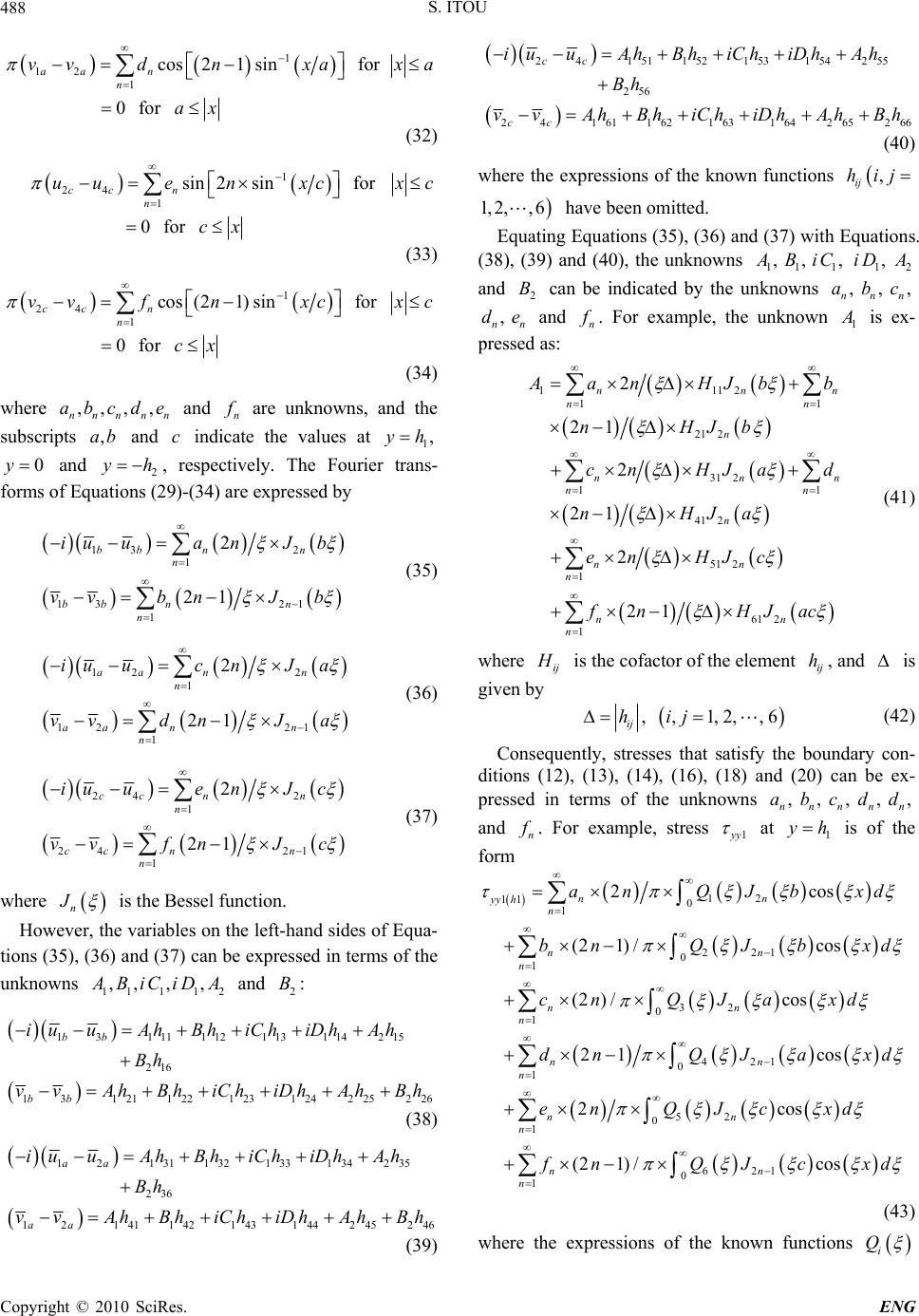 S. ITOU 488 1 12 1cos21sinfor 0for aan n vv dnxax ax a (32) 1 24 1sin2sinfor 0for ccn n uuenxcx cx c (33) 1 24 1cos(21) sinfor 0for cc n n vvf nxcx cx c (34) where and ,,,, nnnnn abcde n f are unknowns, and the subscripts and indicate the values at ,ab c1,yh and , respectively. The Fourier trans- forms of Equations (29)-(34) are expressed by 0y2 yh 13 2 1 13 21 1 2 21 bb nn n bb nn n iuuanJ b vvbnJ b (35) 12 2 1 12 21 1 2 21 aa nn n aa nn n iuucnJ a vvdnJ a (36) 24 2 1 24 21 1 2 21 cc nn n cc nn n iuuenJc vvfnJc (37) where n J is the Bessel function. However, the variables on the left-hand sides of Equa- tions (35), (36) and (37) can be expressed in terms of the unknowns 11 112 ,, ,, A BiCiDA and : 2 B 13111112 113 114215 216 131 211 221 231 24225226 bb bb iuuAh BhiCh iDhAh Bh vv AhBhiChiDhAhBh (38) 121311 321 331342 35 236 121 411 421 431 44245246 aa aa iu uAh Bh iChiDhAh Bh vv AhBhiChiDhAhBh (39) 24151152 153 154255 256 241 611621 631 64265266 cc cc iuuAh Bh iCh iDhAh Bh vv AhBhiChiDhAhBh (40) where the expressions of the known functions , ij hij have been omitted. 1, 2,, 6 Equating Equations (35), (36) and (37) with Equations. (38), (39) and (40), the unknowns 1, A 1,B1,iC1,iD 2 A and can be indicated by the unknowns and 2 B n e , n a, n bc , n , n dn f . For example, the unknown 1 A is ex- pressed as: 1112 11 21 2 31 2 11 41 2 51 2 1 61 2 1 2 21 2 21 2 21 nn nn n nn nn n nn n nn n n n A anHJb b nHJb cnHJa d nHJa en HJc fn HJac (41) where ij H is the cofactor of the element , and ij h is given by ,, 1,2,,6 ij hij (42) Consequently, stresses that satisfy the boundary con- ditions (12), (13), (14), (16), (18) and (20) can be ex- pressed in terms of the unknowns and , n a, n b, n c, n d, n d n f . For example, stress 1 y y at is of the form 1 yh 12 11 0 1 221 0 1 32 0 1 421 0 1 52 0 1 621 2c (2 1)/cos (2 )/cos 21 cos 2cos (2 1)/co nn yy hn nn n nn n nn n nn n nn anQJb xd bnQJbxd cnQJa xd dnQJ axd enQJcxd fnQJc os 0 1s n x d (43) where the expressions of the known functions i Q Copyright © 2010 SciRes. ENG  S. ITOU489 1,2,, 6i have been omitted. Finally, the remaining boundary conditions (15), (17) and (19), which must be satisfied inside the cracks, reduce to the forms: 11 15 nn nn aFx eF 1213 14 11 11 16 1 11 for nnnn nn nn nn nn nn bFxcFx dFx xfFxu xxb (44) 21 25 nn nn aFx eF 2223 24 11 11 26 2 11 for nnnn nn nn nn nn nn bFxcFx dFx xfFxu xxb (45) 31 35 nn nn aF x eF 32 33 34 11 11 36 3 11 for nnnnnn nn nn nn nn bF xcF xdF x xfFxu xxa (46) 41 45 nn nn aFx eF 4243 44 11 11 46 4 11 ()for nnnn nn nn nn nn nn bFxcFx dFx xfFxu xxa (47) 51 55 nn nn aF x eF 52 53 54 11 11 56 5 11 for nnnnnn nn nn nn nn bF xcF xdF x xfFxu xxc (48) 61 65 nn nn aF x eF 6263 64 11 11 66 6 11 for nnnn nn nn nn nn nn bF xcF xdF x xfFxu xxc (49) where the functions are known. For example, ,1,2,,6 nij Fxij , 11n F x 12n F x66n and F x are ex- pressed as 111 2 0 2cos nn F xn QJbxd (50) 222 1 0 22 1 2 21 cos21sin nLn L nQQJ b 12 cos Fx x dQ bxnxb (51) 66362 1 0 21 sin nn F xnQJc xd (52) where the constant 2 L Q is given by 22 L L QQ (53) where L is a larger value of . The functions i ux are denoted by the equations: 1123 45 26 exp ,0,, 0,exp ,0 ux pihuxux p uxuxpihux (54) The unknowns and ,,,, nnn nn abcde n f in Equations (44), (45), (46), (47), (48) and (49) can now be solved using the Schmidt method described in Appendix A. 4. Stress Intensity Factors Once the unknown coefficients and ,,,, nnnnn abcde n f have been solved, all the stresses and displacements can likewise be solved. In fracture mechanics, it is important to determine the stress intensity factors defined from the stresses in the region near the crack ends. Using the rela- tions 0 1/2 1/2 22 22 1/2 1/2 22 22 cos, sin sin , cos n n n n n Jax xd ax ax x an ax axx anforax (55) the stress intensity factors can be expressed as 1 11(1 2 1 1 21(1 7 1 lim 2 21 1 lim 2 21 hyy h xb n nL n hxy h xb n nL n Kxb bn Q Kxb anQ b ) ) b (56) 0 11(0) 16 1 0 21(0) 21 1 lim2 () 21(1) lim 2 21 yy xa n nL n xy xa n nL n Kxa dn Q Kxa cnQ a a (57) Copyright © 2010 SciRes. ENG 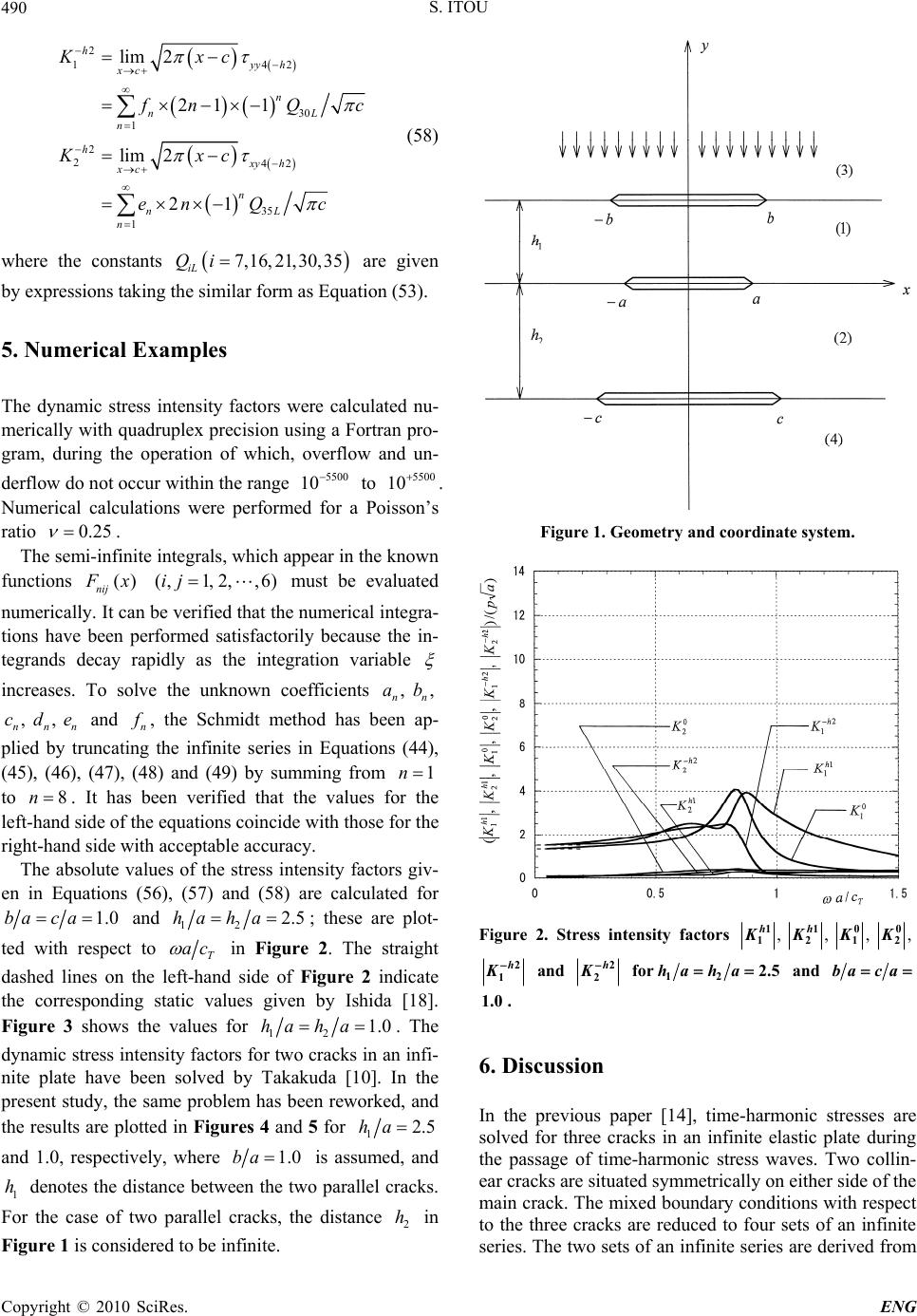 S. ITOU 490 2 142 30 1 2 242 35 1 lim 2 21 1 lim 2 21 hyy h xc n nL n hxy h xc n nL n Kxc f nQ Kxc enQ c c (58) where the constants are given by expressions taking the similar form as Equation (53). 7,16,21,30,35 iL Qi 5. Numerical Examples The dynamic stress intensity factors were calculated nu- merically with quadruplex precision using a Fortran pro- gram, during the operation of which, overflow and un- derflow do not occur within the range to . Numerical calculations were performed for a Poisson’s ratio 5500 105500 10 0.25 . The semi-infinite integrals, which appear in the known functions () nij F x must be evaluated numerically. It can be verified that the numerical integra- tions have been performed satisfactorily because the in- tegrands decay rapidly as the integration variable (,1,2, ,6)ij increases. To solve the unknown coefficients and , n a, n b , n c, n dn en f , the Schmidt method has been ap- plied by truncating the infinite series in Equations (44), (45), (46), (47), (48) and (49) by summing from 1n to . It has been verified that the values for the left-hand side of the equations coincide with those for the right-hand side with acceptable accuracy. 8n The absolute values of the stress intensity factors giv- en in Equations (56), (57) and (58) are calculated for 1.0ba ca and 12 2.5ha ha; these are plot- ted with respect to T ac in Figure 2. The straight dashed lines on the left-hand side of Figure 2 indicate the corresponding static values given by Ishida [18]. Figure 3 shows the values for 12 1.0ha ha. The dynamic stress intensity factors for two cracks in an infi- nite plate have been solved by Takakuda [10]. In the present study, the same problem has been reworked, and the results are plotted in Figures 4 and 5 for 12.5ha and 1.0, respectively, where 1.0ba is assumed, and denotes the distance between the two parallel cracks. For the case of two parallel cracks, the distance in Figure 1 is considered to be infinite. 1 h 2 h Figure 1. Geometry and coordinate system. Figure 2. Stress intensity factors , 1 1 h K, 1 2 h K, 0 1 K, 0 2 K 2 1h K and 2 2h K for12 2.5ha ha and ba ca . 1.0 6. Discussion In the previous paper [14], time-harmonic stresses are solved for three cracks in an infinite elastic plate during the passage of time-harmonic stress waves. Two collin- ear cracks are situated symmetrically on either side of the main crack. The mixed boundary conditions with respect to the three cracks are reduced to four sets of an infinite series. The two sets of an infinite series are derived from Copyright © 2010 SciRes. ENG 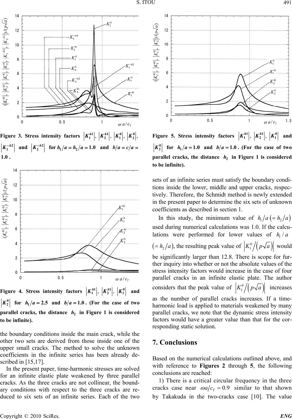 S. ITOU491 Figure 3. Stress intensity factors , 1 1 h K, 1 2 h K, 0 1 K, 0 2 K 2 1h K and 2 2h K for12 1.0ha ha and ba ca . 1.0 Figure 4. Stress intensity factors , 1 1 h K, 1 2 h K0 1 K and 0 2 K for 12.5ha and 1.0ba . (For the case of two parallel cracks, the distance in Figure 1 is considered to be infinite). 2 h the boundary conditions inside the main crack, while the other two sets are derived from those inside one of the upper small cracks. The method to solve the unknown coefficients in the infinite series has been already de- scribed in [15,17]. In the present paper, time-harmonic stresses are solved for an infinite elastic plate weakened by three parallel cracks. As the three cracks are not collinear, the bound- ary conditions with respect to the three cracks are re- duced to six sets of an infinite series. Each of the two Figure 5. Stress intensity factors , 1 1 h K, 1 2 h K0 1 K and 0 2 K for 11.0ha and 1.0ba. (For the case of two parallel cracks, the distance in Figure 1 is considered to be infinite). 2 h sets of an infinite series must satisfy the boundary condi- tions inside the lower, middle and upper cracks, respec- tively. Therefore, the Schmidt method is newly extended in the present paper to determine the six sets of unknown coefficients as described in section 1. In this study, the minimum value of 12 ha ha used during numerical calculations was 1.0. If the calcu- lations were performed for lower values of 1/ha 2 ha, the resulting peak value of 0 1 K pa would be significantly larger than 12.8. There is scope for fur- ther inquiry into whether or not the absolute values of the stress intensity factors would increase in the case of four parallel cracks in an infinite elastic plate. The author considers that the peak value of 0 1 K pa increases as the number of parallel cracks increases. If a time- harmonic load is applied to materials weakened by many parallel cracks, we note that the dynamic stress intensity factors would have a greater value than that for the cor- responding static solution. 7. Conclusions Based on the numerical calculations outlined above, and with reference to Figures 2 through 5, the following conclusions are reached: 1) There is a critical circular frequency in the three cracks case near 0.9 T ac similar to that shown by Takakuda in the two-cracks case [10]. The value Copyright © 2010 SciRes. ENG  S. ITOU Copyright © 2010 SciRes. ENG 492 0 1 K pa is 12.8 for 12 1.0ha ha. For two parallel cracks, the corresponding value is 5.87. It can be seen that the presence of the third crack has a significant effect upon the dynamic stress intensity factor around the center crack between the upper and lower parallel cracks. [7] S. Itou, “Dynamic Stress Concentration around Two Co- planar Griffith Cracks in an Infinite Elastic Medium,” ASME Journal of Applied Mechanics, Vol. 45, No. 12, 1978, pp. 803-806. [8] S. Itou, “Diffraction of an Antiplane Shear Wave by Two Coplanar Griffith Cracks in an Infinite Elastic Medium,” International Journal of Solids and Structures, Vol. 16, No. 12, 1980, pp. 1147- 1153. 2) For 12 2.5ha ha (Figure 2), the slope to the peak value of 0 1 K pa is comparatively gentle. However, for 12 1.0ha ha (Figure 3), the curve rises steeply to the maximum value of 0 1 K pa , after which it declines equally steeply. The curve exhib- its a sharp peak at the critical circular frequency near 0.9 T ac . [9] S. Itou, “Dynamic Stresses around Two Cracks Placed Symmetrically to a Large Crack,” International Journal of Fracture, Vol. 75, No. 3, 1996, pp. 261-271. [10] K. Takakuda, “Scattering of Plane Harmonic Waves by Cracks (in Japanese),” Transactions of Japan Society of Mechanical Engineeris, Series A, Vol. 48, No. 432, 1982, pp. 1014-1020. [11] H. So and J. Y. Huang, “Determination of Dynamic Stress Intensity Factors of Two Finite Cracks at Arbi- trary Positions by Dislocation Model,” International Journal of Engineering Science, Vol. 26, No. 2, 1988, pp. 111-119. 3) In static solutions, the stress intensity factors for three equal-length cracks decrease slightly as 1 ha 2 ha decreases. However, this is accompanied by a significant increase in the peak value of 0 1 K pa. [12] S. A. Meguid and X. D. Wang, “On the Dynamic Interac- tion between a Microdefect and a Main Crack,” Pro- ceedings of the Royal Society of London, Series A, Vol. 448, No. 1934, 1995, pp. 449-464. 8. References [13] M. Ayatollahi and S. J. Fariborz, “Elastodynamic Analy- sis of a Plane Weakened by Several Cracks,” Interna- tional Journal of Solids and Structures, Vol. 46, No. 7-8, 2009, pp. 1743-1754. [1] J. F. Loeber and G. C. Sih, “Diffraction of Antiplane Shear by a Finite Crack,” Journal of the Acoustical Soci- ety of America, Vol. 44, No. 1, 1968, pp. 90-98. [14] S. Itou and H. Haliding, “Dynamic Stress Intensity Fac- tors around Three Cracks in an Infinite Elastic Plane Subjected to Time-Hharmonic Stress Waves,” Interna- tional Journal of Fracture, Vol. 83, No. 4, 1997, pp. 379- 391. [2] G. C. Sih and J. F. Loeber, “Wave Propagation in an Elastic Solid with a Line of Discontinuity or Finite Crack,” Quarterly of Applied Mathematics, Vol. 27, No. 2, 1969, pp. 193-213. [15] S. Itou and H. Haliding, “Dynamic Stress Intensity Fac- tors around Two Parallel Cracks in an Infinite-Orth- otropic Plane Subjected to Incident Harmonic Stress Wa v es, ” International Journal of Solids and Structures, Vol. 34, No. 9, 1997, pp. 1145-1165. [3] A. K. Mal, “Interaction of Elastic Waves with a Griffith Crack,” International Journal of Engineering Science, Vol. 8, No. 9, 1970, pp. 763-776. [4] G. C. Sih and J. F. Loeber, “Torsional Vibration of an Elastic Solid Containing a Penny-Shaped Crack,” Journal of the Acoustical Society of America, Vol. 44, No. 5, 1968, pp. 1237-1245. [16] P. M. Morse and H. Feshbach, “Methods of Theoretical Physics,” McGraw-Hill, New York, Vol. 1, 1958. [17] S. Itou, “Axisymmetric Slipless Indentation of an Infinite Elastic Hollow Cylinder,” Bulletin of the Calcutta Ma- thematical Society, Vol. 68, No. 17, 1976, pp. 157-165. [5] G. C. Sih and J. F. Loeber, “Normal Compression and Radial Shear Waves Scattering at a Penny-Shaped Crack in an Elastic Solid,” Journal of the Acoustical Society of America, Vol. 46, No. 3B, 1969, pp. 711-721. [18] M. Ishida, “Elastic Analysis of Cracks and Stress In- tensity Factors (in Japanese),” Fracture Mechanics and Strength of Materials, Baifuukan Press, Tokyo, Vol. 2, 1976. [6] A. K. Mal, “Interaction of Elastic Waves with a Penny- Shaped Crack,” International Journal of Engineering Science, Vol. 8, No. 5, 1970, pp. 381-388.  S. ITOU 493 Appendix A For convenience, Equations (42) through (47) can be rewritten as 11 121314 11 11 15161 11 for nn nnnnnn nn nn nn nn nn aFx bFxcFx dFx eFxfFxu xxb (A.1) 21 222324 11 11 2526 2 11 for nn nnnnnn nn nn nn nn nn aFx bFxcFxdFx eFxfFxu xxb (A.2) 31 323334 11 11 3536 3 11 for nn nnnnnn nn nn nn nn nn aF xbFxcF xdFx eFxfFxu xxa (A.3) 41 424344 11 11 4546 4 11 for nn nnnnnn nn nn nn nn nn aFx bFxcFxdFx eFxfFxu xxa (A.4) 51 525354 11 11 5556 5 11 for nn nnnnnn nn nn nn nn nn aF xbFxcF xdFx eFxfFxu xxc (A.5) 61 626364 11 11 6566 6 11 for nn nnnnnn nn nn nn nn nn aF xbFxcFxdFx eFxfFxu xxc (A.6) A set of functions that satisfy the orthogonal- ity condition () n Gx 2 00 , bb mnnmnn n GxGx dxIIGx dx (A.7) can be constructed from a given set of arbitrary function, say 65() n F x, such that 65 1 n ninnni i GxPPFx (A.8) where is the cofactor of the element of , which is defined as in Pin d' n D 11 121 21 65 65 0 1 ', n c nini nnn ddd d DdFx dd n Fxdx (A.9) Representing the fifth series in Equation (A.6) by the orthogonal series with coefficients () n Gx n , the fol- lowing relationships are derivable: 65 11 66162 11 1 64 66 11 nnn n nn nn nnnn nn n nn nn nn eFxG x uxaF xbF xcF x dF xfF x 63 (A.10) The second equality yields 66 00 1 62 63 00 11 64 66 00 11 1 for cc nn ini i n cc in iini ii cc in iini ii Gxuxdxa GxFxdx I bGxFxdx cGxFxdx dGxFxdx fGxFxdx xc 1 (A.11) and considering Equation (A.8), the first equality shows that 0 11111 abc d nniniiniiniinii ni iiiii eabcd f f (A.12) with 06 0 61 0 62 0 63 0 64 0 66 0 , , , , , c nj nj jn jj j c nj a nij i jn jj j c nj b nij i jn jj j c nj c nij i jn jj j c nj d nij i jn jj j c nj f nij i jn jj j PGxuxdx PI PGxF xdx PI PGxF xdx PI PGxF xdx PI PGxF xdx PI PGxF xdx PI (A.13) Copyright © 2010 SciRes. ENG  S. ITOU 494 Substituting Equation (A.12) into Equation (A.5), the equality now becomes ** 51 5253 11 1 *** 5456 5 11 for nn nnnn nn n nn nn nn aF xbFxcF x dF xfF xux xc * (A.14) with * 51 5155 1 * 52 5255 1 * 53 5355 1 * 54 5455 1 * 56 5655 1 *0 55 55 1 , , , , , a nn ini i b nn ini i c nn ini i d nn ini i f nn ini i ii i F xFx Fx F xFx Fx F xFx Fx F xFx Fx F xFx Fx ux uxFx (A.15) Using the same procedure, the orthogonal function *() n H x is constructed from * 56 () n F x as ** 56 1 n ninnni i H xQQF x (A.16) where is the cofactor of the element in Qin g of , which is defined as '' n D 11 121 21 1 ** 56 56 0 '' , n n nn c in in gg g g D gg n g FxFxdx (A.17) Using Equations (A.14) and (A.16), the coefficient n f can be expressed by and as follows: ,, nnn abcn d 0 11 11 ab nniniini ii cd iniini ii fa cd b (A.18) with 0** 5 0 ** 51 0 ** 52 0 ** 53 0 ** 54 0 2 * 0 , , , , , c nj nj jn jj j c nj a nij i jn jj j c nj b nij i jn jj j c nj c nij i jn jj j c nj d nij i jn jj j c nn Q H xu xdx QJ Q H xF xdx QJ Q H xF xdx QJ Q H xF xdx QJ Q H xF xdx QJ JHxdx (A.19) Substituting Equation (A18) into Equation (A12), we obtain the following relation: 0*** 11 ** 11 ab nnini ini ii cd iniini ii eab cd (A.20) with 0* 00 1 * 1 * 1 * 1 * 1 , , , , f nn jnj j aa af ninijinj j bb bf niniji nj j cc cf niniji nj j dd d niniji nj j f (A.21) Replacing the coefficients and n en f in Equations (A.1), (A.2), (A.3) and (A.4) with Equations (A.18) and (A.20), the equality becomes ** 11 1213 11 1 ** 14 1 1for nn nnnn nn n nn n aF xbFxcF x dFxuxxb * (A.22) ** * 21 2223 11 1 ** 24 2 1for nn nnnn nnn nn n aF xbF xcFx dFxuxxb (A.23) Copyright © 2010 SciRes. ENG  S. ITOU Copyright © 2010 SciRes. ENG 495 ** 31 3233 11 1 ** 34 3 1for nn nnnn nn n nn n aF xbFxcF x dFxuxxa * (A.24) ** 41 4243 111 ** 44 4 1for nn nnnn nnn nn n aF xbF xcFx dFxu xxa * (A.25) with ** 11 111516 1 ** 12 151516 1 ** 13 131516 1 ** 14 141516 1 *0* 11 15 1 , , , , aa nn iniini i bb nn iniini i cc nn iniini i dd nn iniini i ii i i FxFxFx Fx F xFxFx Fx FxFxFxFx F xFxFx Fx uxuxF x 016i Fx (A.26) ** 31 313536 1 ** 32 353536 1 ** 33 333536 1 ** 34 343536 1 *0* 33 35 1 , , , , aa nn iniini i bb nn iniini i cc nn iniini i dd nn iniini i iii i F xFxFx Fx F xFxFx Fx F xFxFx Fx F xFxFx Fx ux uxF x 036 i Fx (A.28) ** 21 212526 1 ** 22 252526 1 ** 23 232526 1 ** 24 242526 1 *0* 22 25 1 , , , , aa nn iniini i bb nn iniini i cc nn iniini i dd nn iniini i iii i F xFxFxFx F xFxFx Fx F xFxFx Fx F xFxFx Fx ux uxF x 026 i Fx (A.27) ** 41 414546 1 ** 42 454546 1 ** 43 434546 1 ** 44 444546 1 *0* 44 45 1 , , , , aa nn iniini i bb nn iniini i cc nn iniini i dd nn iniini i iii i F xFxFxFx F xFxFxFx F xFxFx Fx F xFxFxFx ux uxF x 046 i Fx (A.29) Equations (A.2 2) , (A. 23 ), (A.24) and (A.25 ) have been already solved for and in Ref. [17, 1 5] . ,, nnn abcn d |