Paper Menu >>
Journal Menu >>
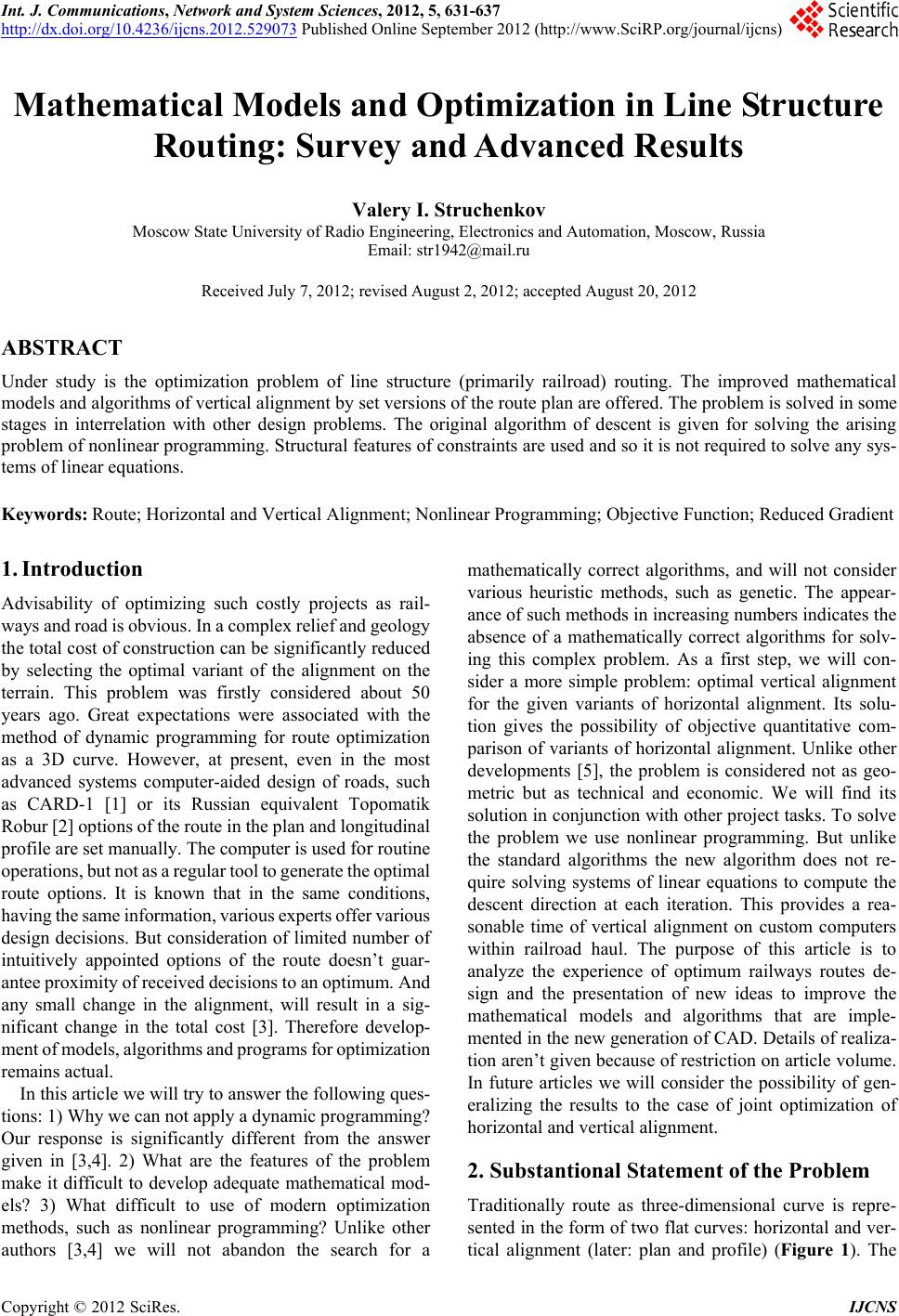 Int. J. Communications, Network and System Sciences, 2012, 5, 631-637 http://dx.doi.org/10.4236/ijcns.2012.529073 Published Online September 2012 (http://www.SciRP.org/journal/ijcns) Mathematical Models and Optimization in Line Structure Routing: Survey and Advanced Results Valery I. Struchenkov Moscow State University of Radio Engineering, Electronics and Automation, Moscow, Russia Email: str1942@mail.ru Received July 7, 2012; revised August 2, 2012; accepted August 20, 2012 ABSTRACT Under study is the optimization problem of line structure (primarily railroad) routing. The improved mathematical models and algorithms of vertical alignment by set versions of the route plan are offered. The problem is solved in some stages in interrelation with other design problems. The original algorithm of descent is given for solving the arising problem of nonlinear programming. Structural features of constraints are used and so it is not required to solve any sys- tems of linear equations. Keywords: Route; Horizontal and Vertical Alignment; Nonlinear Programming; Objective Function; Reduced Gradient 1. Introduction Advisability of optimizing such costly projects as rail- ways and road is obvious. In a complex relief and geology the total cost of construction can be significantly reduced by selecting the optimal variant of the alignment on the terrain. This problem was firstly considered about 50 years ago. Great expectations were associated with the method of dynamic programming for route optimization as a 3D curve. However, at present, even in the most advanced systems computer-aided design of roads, such as CARD-1 [1] or its Russian equivalent Topomatik Robur [2] options of the route in the plan and longitudinal profile are set manually. The computer is used for routine operations, but not as a regular tool to generate the optimal route options. It is known that in the same conditions, having the same information, various experts offer various design decisions. But consideration of limited number of intuitively appointed options of the route doesn’t guar- antee proximity of received decisions to an optimum. And any small change in the alignment, will result in a sig- nificant change in the total cost [3]. Therefore develop- ment of models, algorithms and programs for optimization remains actual. In this article we will try to answer the following ques- tions: 1) Why we can not apply a dynamic programming? Our response is significantly different from the answer given in [3,4]. 2) What are the features of the problem make it difficult to develop adequate mathematical mod- els? 3) What difficult to use of modern optimization methods, such as nonlinear programming? Unlike other authors [3,4] we will not abandon the search for a mathematically correct algorithms, and will not consider various heuristic methods, such as genetic. The appear- ance of such methods in increasing numbers indicates the absence of a mathematically correct algorithms for solv- ing this complex problem. As a first step, we will con- sider a more simple problem: optimal vertical alignment for the given variants of horizontal alignment. Its solu- tion gives the possibility of objective quantitative com- parison of variants of horizontal alignment. Unlike other developments [5], the problem is considered not as geo- metric but as technical and economic. We will find its solution in conjunction with other project tasks. To solve the problem we use nonlinear programming. But unlike the standard algorithms the new algorithm does not re- quire solving systems of linear equations to compute the descent direction at each iteration. This provides a rea- sonable time of vertical alignment on custom computers within railroad haul. The purpose of this article is to analyze the experience of optimum railways routes de- sign and the presentation of new ideas to improve the mathematical models and algorithms that are imple- mented in the new generation of CAD. Details of realiza- tion aren’t given because of restriction on article volume. In future articles we will consider the possibility of gen- eralizing the results to the case of joint optimization of horizontal and vertical alignment. 2. Substantional Statement of the Problem Traditionally route as three-dimensional curve is repre- sented in the form of two flat curves: horizontal and ver- tical alignment (later: plan and profile) (Figure 1). The C opyright © 2012 SciRes. IJCNS 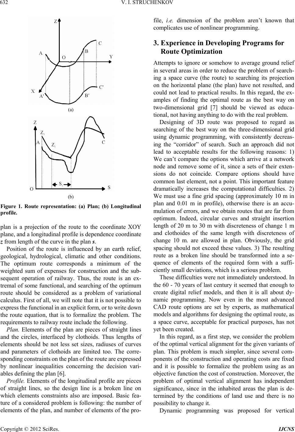 V. I. STRUCHENKOV 632 (a) (b) Figure 1. Route representation: (a) Plan; (b) Longitudinal profile. plan is a projection of the route to the coordinate XOY plane, and a longitudinal profile is dependence coordinate z from length of the curve in the plan s. Position of the route is influenced by an earth relief, geological, hydrological, climatic and other conditions. The optimum route corresponds a minimum of the weighted sum of expenses for construction and the sub- sequent operation of railway. Thus, the route is an ex- tremal of some functional, and searching of the optimum route should be considered as a problem of variational calculus. First of all, we will note that it is not possible to express the functional in an explicit form, or to write down the route equation, that is to formalize the problem. The requirements to railway route include the following. Plan. Elements of the plan are pieces of straight lines and the circles, interfaced by clothoids. Thus lengths of elements should be not less set sizes, radiuses of curves and parameters of clothoids are limited too. The corre- sponding constraints on the plan of the route are expressed by nonlinear inequalities concerning the decision vari- ables defining the plan [6]. Profile. Elements of the longitudinal profile are pieces of straight lines, so the design line is a broken line on which elements constraints also are imposed. Basic fea- ture of a considered problem is following: the number of elements of the plan, and number of elements of the pro- file, i.e. dimension of the problem aren’t known that complicates use of nonlinear programming. 3. Experience in Developing Programs for Route Optimization Attempts to ignore or somehow to average ground relief in several areas in order to reduce the problem of search- ing a space curve (the route) to searching its projection on the horizontal plane (the plan) have not resulted, and could not lead to practical results. In this regard, the ex- amples of finding the optimal route as the best way on two-dimensional grid [7] should be viewed as educa- tional, not having anything to do with the real problem. Designing of 3D route was proposed to regard as searching of the best way on the three-dimensional grid using dynamic programming, with consistently decreas- ing the “corridor” of search. Such an approach did not lead to acceptable results for the following reasons: 1) We can’t compare the options which arrive at a network node and remove some of it, since a sets of their exten- sions do not coincide. Compare options should have common last element, not a point. This important feature dramatically increases the computational difficulties. 2) We must use a fine grid spacing (approximately 10 m in plan and 0.01 m in profile), otherwise there is an accu- mulation of errors, and we obtain routes that are far from optimum. Indeed, circular curves and straight insertion length of 20 m to 30 m with discreteness of change 1 m and clothoides of the same length with discreteness of change 10 m. are allowed in plan. Obviously, the grid spacing should not exceed these values. 3) The resulting route as a broken line should be transformed into a se- quence of elements of the required form with a suffi- ciently small deviations, which is a serious problem. These difficulties were not immediately understood. In the 60 - 70 years of last century it seemed that enough to create digital relief models, and then it is all about dy- namic programming. Now even in the most advanced CAD route options are set by experts, as mathematical models and algorithms for designing the optimal route, as a space curve, acceptable for practical purposes, has not yet been created. In this regard, as a first step, we consider the problem of the optimal vertical alignment for the given variants of plan. This problem is much simpler, since several com- ponents of the construction and operating costs are fixed and it is possible to formalize the problem using as an objective function the cost of construction. Moreover, the problem of optimal vertical alignment has independent significance, since in the inhabited areas the plan is de- termined by the conditions of land use and there is no possibility to change it. Dynamic programming was proposed for vertical Copyright © 2012 SciRes. IJCNS 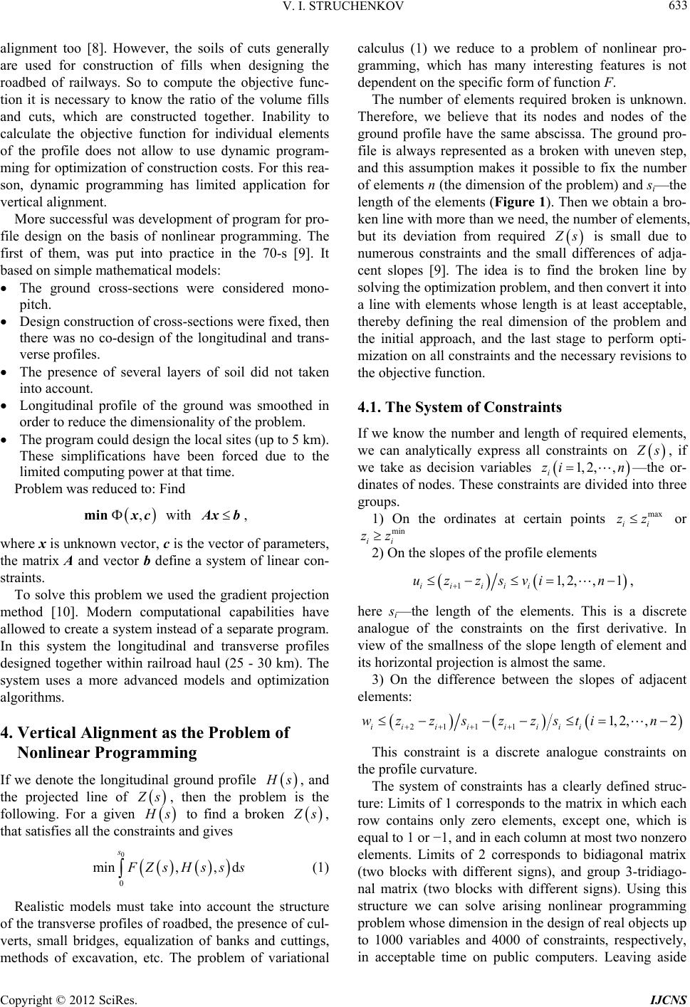 V. I. STRUCHENKOV 633 alignment too [8]. However, the soils of cuts generally are used for construction of fills when designing the roadbed of railways. So to compute the objective func- tion it is necessary to know the ratio of the volume fills and cuts, which are constructed together. Inability to calculate the objective function for individual elements of the profile does not allow to use dynamic program- ming for optimization of construction costs. For this rea- son, dynamic programming has limited application for vertical alignment. More successful was development of program for pro- file design on the basis of nonlinear programming. The first of them, was put into practice in the 70-s [9]. It based on simple mathematical models: The ground cross-sections were considered mono- pitch. Design construction of cross-sections were fixed, then there was no co-design of the longitudinal and trans- verse profiles. The presence of several layers of soil did not taken into account. Longitudinal profile of the ground was smoothed in order to reduce the dimensionality of the problem. The program could design the local sites (up to 5 km). These simplifications have been forced due to the limited computing power at that time. Problem was reduced to: Find Ф,xcmin Ax b with , where x is unknown vector, c is the vector of parameters, the matrix A and vector b define a system of linear con- straints. To solve this problem we used the gradient projection method [10]. Modern computational capabilities have allowed to create a system instead of a separate program. In this system the longitudinal and transverse profiles designed together within railroad haul (25 - 30 km). The system uses a more advanced models and optimization algorithms. 4. Vertical Alignment as the Problem of Nonlinear Programming If we denote the longitudinal ground profile H s , and the projected line of Z s , then the problem is the following. For a given H s to find a broken Z s ,, d , that satisfies all the constraints and gives 0 0 min s F Zs Hs ss (1) Realistic models must take into account the structure of the transverse profiles of roadbed, the presence of cul- verts, small bridges, equalization of banks and cuttings, methods of excavation, etc. The problem of variational calculus (1) we reduce to a problem of nonlinear pro- gramming, which has many interesting features is not dependent on the specific form of function F. The number of elements required broken is unknown. Therefore, we believe that its nodes and nodes of the ground profile have the same abscissa. The ground pro- file is always represented as a broken with uneven step, and this assumption makes it possible to fix the number of elements n (the dimension of the problem) and si—the length of the elements (Figure 1). Then we obtain a bro- ken line with more than we need, the number of elements, but its deviation from required Z s is small due to numerous constraints and the small differences of adja- cent slopes [9]. The idea is to find the broken line by solving the optimization problem, and then convert it into a line with elements whose length is at least acceptable, thereby defining the real dimension of the problem and the initial approach, and the last stage to perform opti- mization on all constraints and the necessary revisions to the objective function. 4.1. The System of Constraints If we know the number and length of required elements, we can analytically express all constraints on Z s 1, 2,,zin max ii zz min i zz , if we take as decision variables i—the or- dinates of nodes. These constraints are divided into three groups. 1) On the ordinates at certain points or i 2) On the slopes of the profile elements 11, 2,,1 ii iii uzzsvi n , here si—the length of the elements. This is a discrete analogue of the constraints on the first derivative. In view of the smallness of the slope length of element and its horizontal projection is almost the same. 3) On the difference between the slopes of adjacent elements: 2111 1,2,,2 iii ii iii wzz sz zstin This constraint is a discrete analogue constraints on the profile curvature. The system of constraints has a clearly defined struc- ture: Limits of 1 corresponds to the matrix in which each row contains only zero elements, except one, which is equal to 1 or −1, and in each column at most two nonzero elements. Limits of 2 corresponds to bidiagonal matrix (two blocks with different signs), and group 3-tridiago- nal matrix (two blocks with different signs). Using this structure we can solve arising nonlinear programming problem whose dimension in the design of real objects up to 1000 variables and 4000 of constraints, respectively, in acceptable time on public computers. Leaving aside Copyright © 2012 SciRes. IJCNS  V. I. STRUCHENKOV 634 the question of concrete models of the objective function and hence the algorithm for computing its gradient, we consider how the new algorithm uses the structure of system constraints. The well-known algorithms of nonlinear programming with linear constraints consist of the following steps: 1) Construction of allowed initial approach z0; 2) Calculation of the gradient of the objective function f 0; 3) Defining a set of active constraints; 4) Construction of the descent direction p0 in the bounding hyperplane; 5) Checking conditions for termination of accounts and, if they are satisfied then stop else following step; 6) Calculate step and a new iterative point 1kkk zzp 1 ТТ ААА Аf – Т рССf ,0 Т f0 and to item 2; For a convex objective function process terminates in the neighborhood of minimum point. Known algorithms differ in the construction of descent direction [10,11]. If as descent direction we accept the projection p of antigradient −f, then the standard algorithm requires solv- ing systems of linear equations of large dimension. The duration of an iteration process for large-scale prob- lems is unacceptable. By Rozen formula [10] pE (2) Here E is the identity matrix and A consists of rows original matrix corresponding to the active (at a given iteration) constraints and the icon T denotes transposition. In the previously developed software several systems of linear equations of small dimension solved to calculate the projection p, instead of one system with the matrix ААТ [9]. However, the features of constraints allow to construct a basis in the corresponding bounding hyperplane and find a descent direction without solving systems of linear equations at all. It can be done with any combination of active constraints. The new algorithm is based on this. Indeed, suppose that we know this basis, and its columns form a matrix C. Block structure matrix of con- straints often allows to calculate the descent direction sequentially by groups of variables, since some variables may be free in the current iteration and therefore the matrix of active constraints contains non-overlapping blocks. As descent direction in the new algorithm adopted —that is reduced antigradient [10,11]. For its calculation is enough to construct only the basis vectors, to calculate СТf, and then multiply С on the result. ,, ТТ рfСС ffСС f if f р ,0 Tab . Consequently, is a descent direction, which can be used instead of antigradient projection. In item 4 of the algorithm, we check the possibility of removing some of the constraints from active set. For this purpose the standard algorithm [10,11] requires solving the systems of linear equations. In the new algo- rithm, instead, we consistently construct vectors, each of which breaks one and only one constraint. These vectors (matrix B) form a basis in the orthogo- nal complement to the null space of A, and together with the vectors of C gives a complete basis. In this basis the matrix of active constraints is diagonal, which simplifies the problem. For example, for the i-th constraint a vector bi is constructed. Since the scalar product ii, then this constraint can be removed from the active set if ,0bf i [12]. Here ai-i-th row of the matrix of active constraints, and f-gradient of the objective function. This rule should be applied to all vectors, each of which breaks one and only one constraint. Once we have found a constraint that can be removed, a further search can be stopped. We add the vector bi in the matrix C, recalculate reduced antigradient and continue the opti- mization process. Characteristically, the recalculation of the reduced an- tigradient does not require working with matrices. Just out of each of the j-th component of the existing reduced antigradient subtracted , i bb ji f . It is not difficult, es- pecially since ,bf 1, ,1zzvsi r i is calculated by analyzing the pos- sibility of removing i-th constraint from the active set. It is important to note that in this construction of additional basis vectors we have the ability to remove no one, but several constraints from active set [12]. If we take measures to prevent the “zigzags” [13], this opens up the possibility of quickly generate the required set of active constraints, to accelerate convergence and reduce computation time. Let us return to the analysis of constraints and show how to construct a basis and remove the constraint from active set, as in the rest of the algorithm standard. Let the active set is composed of second types of con- straints (on the slope), i.e. on a railway section is the limiting slope. Then 1iiii . In this case, the dimension of the null - space M matrix of active constraints is equal to 1. For a basis vector сM we have 11,, iirс 1 r . This is shift site. Thus, if p is reduced gradient, then j i i pf , but if p is the projection of the gradient, then 1 r ji i pfr 1, 2,,jr 1kkkk zzvs . The base vector b, which violates only , has the form: i and bi . The constraint is removed if 01,,bi k 11,, ik r 1 ,0 r i ik bf f Copyright © 2012 SciRes. IJCNS 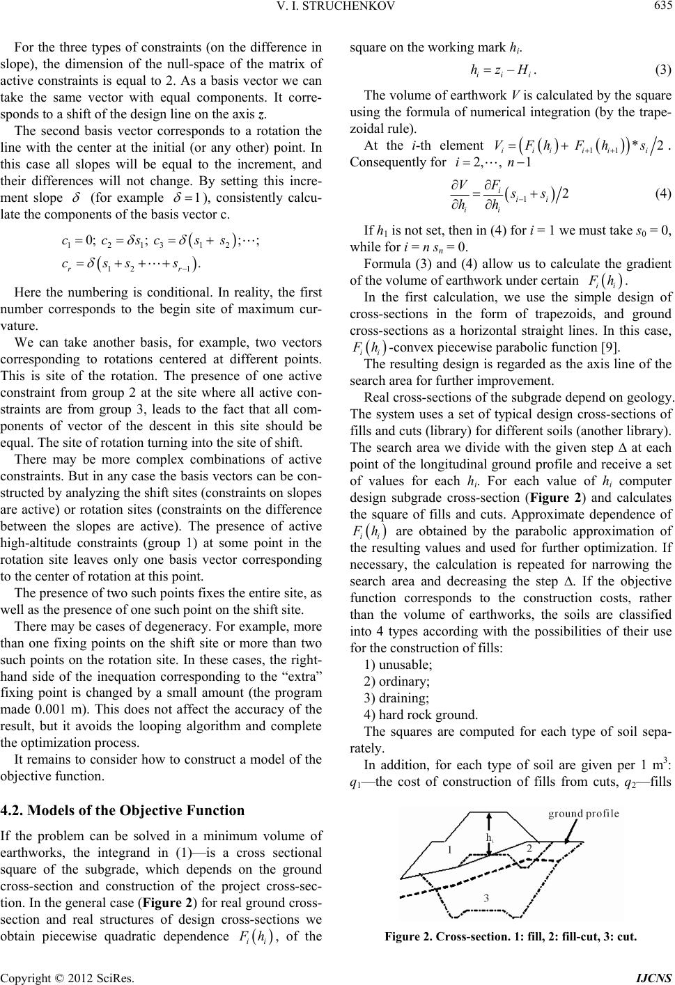 V. I. STRUCHENKOV 635 For the three types of constraints (on the difference in slope), the dimension of the null-space of the matrix of active constraints is equal to 2. As a basis vector we can take the same vector with equal components. It corre- sponds to a shift of the design line on the axis z. The second basis vector corresponds to a rotation the line with the center at the initial (or any other) point. In this case all slopes will be equal to the increment, and their differences will not change. By setting this incre- ment slope (for example 1 12 1 ;; . ss s ii ), consistently calcu- late the components of the basis vector c. 1213 12 0; ; rr ccsc css Here the numbering is conditional. In reality, the first number corresponds to the begin site of maximum cur- vature. We can take another basis, for example, two vectors corresponding to rotations centered at different points. This is site of the rotation. The presence of one active constraint from group 2 at the site where all active con- straints are from group 3, leads to the fact that all com- ponents of vector of the descent in this site should be equal. The site of rotation turning into the site of shift. There may be more complex combinations of active constraints. But in any case the basis vectors can be con- structed by analyzing the shift sites (constraints on slopes are active) or rotation sites (constraints on the difference between the slopes are active). The presence of active high-altitude constraints (group 1) at some point in the rotation site leaves only one basis vector corresponding to the center of rotation at this point. The presence of two such points fixes the entire site, as well as the presence of one such point on the shift site. There may be cases of degeneracy. For example, more than one fixing points on the shift site or more than two such points on the rotation site. In these cases, the right- hand side of the inequation corresponding to the “extra” fixing point is changed by a small amount (the program made 0.001 m). This does not affect the accuracy of the result, but it avoids the looping algorithm and complete the optimization process. It remains to consider how to construct a model of the objective function. 4.2. Models of the Objective Function If the problem can be solved in a minimum volume of earthworks, the integrand in (1)—is a cross sectional square of the subgrade, which depends on the ground cross-section and construction of the project cross-sec- tion. In the general case (Figure 2) for real ground cross- section and real structures of design cross-sections we obtain piecewise quadratic dependence h, of the square on the working mark hi. F – ii i hzH. (3) The volume of earthwork V is calculated by the square using the formula of numerical integration (by the trape- zoidal rule). At the i-th element 11 *2 iii iii hFh s 2,, 1in VF . Consequently for 12 i ii ii F Vss hh (4) If h1 is not set, then in (4) for i = 1 we must take s0 = 0, while for i = n sn = 0. Formula (3) and (4) allow us to calculate the gradient of the volume of earthwork under certain ii F h. In the first calculation, we use the simple design of cross-sections in the form of trapezoids, and ground cross-sections as a horizontal straight lines. In this case, i F i h-convex piecewise parabolic function [9]. The resulting design is regarded as the axis line of the search area for further improvement. Real cross-sections of the subgrade depend on geology. The system uses a set of typical design cross-sections of fills and cuts (library) for different soils (another library). The search area we divide with the given step at each point of the longitudinal ground profile and receive a set of values for each hi. For each value of hi computer design subgrade cross-section (Figure 2) and calculates the square of fills and cuts. Approximate dependence of ii F h are obtained by the parabolic approximation of the resulting values and used for further optimization. If necessary, the calculation is repeated for narrowing the search area and decreasing the step . If the objective function corresponds to the construction costs, rather than the volume of earthworks, the soils are classified into 4 types according with the possibilities of their use for the construction of fills: 1) unusable; 2) ordinary; 3) draining; 4) hard rock ground. The squares are computed for each type of soil sepa- rately. In addition, for each type of soil are given per 1 m3: q1—the cost of construction of fills from cuts, q2—fills Figure 2. Cross-section. 1: fill, 2: fill-cut, 3: cut. Copyright © 2012 SciRes. IJCNS  V. I. STRUCHENKOV 636 from borrow pits (reserves), q3—development unsuitable or excessive soil. The cost of subgrade construction K are calculated through the volumes of fills vf and cuts vc depending on the ratio vf, vc. 1) f c vv 2 12f c . Then 12 cfc K qvq vvqv qq v 2) f c vv 13 3 . Then 13fс f fc K qvqvvqqvqv Development of unsuitable soils is taken into account separately. Characteristically, the coefficients of vf, vc (reduced unit value) vary from iteration to iteration, if the ratio of volumes change. Therefore, at each iteration, we com- pute the corresponding squares and volumes in the whole site and determine the appropriate reduced unit costs for different types of soils. If we specify a reduced unit cost, based on f c, it usually turns out the project line for which vv f c and inversely. That’s why we can’t use dynamic programming. Costs of engineering structures (pipe-culvert, small bridges, etc.) are included in the ob- jective function. For each structure we set the depend- ence of its cost from the working mark (hi). We take into account the possibility to change the types of structures with large changes of the working marks. vv Thus, in the cost model takes into account the rela- tionship of design problems and computer simultane- ously with the design of the longitudinal profile designs cross-sections, and provides a choice of types of engi- neering structures. The calculations are repeated with refinement of the input data. The project line as a result of optimization does not satisfy the constraints on the minimum length of the ele- ment mini s L. But we have reduced limit difference between the slopes of adjacent elements in proportion to reduction of half the sum of their lengths with respect to Lmin. Therefore possible deviations in its transformation to the final form in the current design standards do not exceed 0.4 m. This transformation in a given band of deviations with steps of 0.02 m is performed using the dynamic programming algorithm [14]. The objective function in this case corresponds to the volume of earth- works. The resulting line is needed only as an initial approach. All the calculations were needed only to establish the number of elements (the dimension of the problem) and the initial approach for the final stage of optimization. At this stage, the new decision variables are the ordinates of the project nodes, through which it is easy to calculate project ordinates at all points of the longitudinal ground profile (old variables). Amount of new decision variables, about an order smaller than the old ones. At this stage, we use the same optimization program. We added only conversion of the derivatives of the ob- jective function with respect to the original variables into derivatives with respect to new variables. 5. The Main Results The main results are as follows: 1) We have overcome the difficulties: the unknown dimension of the problem, the lack of analytical expres- sions of the optimality criterion, etc. and formalized the optimal vertical alignment, as a nonlinear programming problem; 2) The proposed mathematical models allow us to de- sign the longitudinal profile simultaneously with the de- sign of the subgrade and the choice of types of pipes and bridges; 3) It is necessary to repeat the calculations with the specification of the model parameters. Therefore need a fast optimization algorithm; 4) The proposed algorithm uses the features of the system of constraints and allows to design the railway haul (25 - 30 km) for 2 - 3 minutes on a standard PC with 2 GHz and 512 MB. 6. Conclusions The developed mathematical models and optimization algorithms allows to solve the problem comprehensively, in the presence data with various completeness and detail, using various criteria. New mathematical model and algorithm co-design of the longitudinal and transverse profiles are the basis of the corresponding subsystem of a new generation of CAD Railway. They can be used for the design of real objects, as well as for research purposes. These models and new algorithm can be used for highways design after a slight modification. REFERENCES [1] CARD/1, 2012. http://www.card-1.com/en/home/ [2] Тоpomatic Robur, 2012. http://www.topomatic.ru [3] Y. Shafahi and M. J. Shahbazi, “Optimum Railway Ali- gnment,” 2012. http://www.uic.org/cdrom/2001/wcrr2001/pdf/sp/2_1_1/2 10.pdf [4] M. K. Jha, P. M. Schonfeld, J.-C. Yong and E. Kim, “In- telligent Road Design,” WIT Press, Southampton, 2006. [5] J. Kurilko and V. Chesheva, “Geonics ZHELDOR- CAD,” CADmaster, Vol. 1, No. 36, 2007. [6] V. I. Struchenkov, “Optimization Methods in Applied Pro- blems,” Solon-Press, Moscow, 2009. Copyright © 2012 SciRes. IJCNS  V. I. STRUCHENKOV Copyright © 2012 SciRes. IJCNS 637 [7] E. S. Wentzel, “Operations Research: Challenges, Prin- ciples, Metodologiya,” KnoRus, Moscow, 2010. [8] V. S. Mikhalevich, V. I. Bykov and A. N. Sibirko, “The Problem of Designing Optimum Longitudinal Profile of the Road,” Transportation Building, Moscow, 1975. [9] Anonym, “The Use of Mathematical Optimization Tech- niques and Computer Engineering at the Longitudinal Profile of the Railways,” Proceedings of the All-Union Scientific Research Institute of Transport Engineering, Transport, Moscow, 1977. [10] F. Gill and W. Murray, “Numerical Methods for Con- strained Optimization,” Mir, Moscow, 1977. [11] M. Aoki, “Introduction to Optimization Methods,” Nauka, Moscow, 1977. [12] V. I. Struchenkov, “Methods for Optimal Design of Routes of Line Structures,” Proceedings of Artificial Intelligence in Engineering Systems, Vol. 20, Gos.IFTP, Moscow, 1999. [13] J. Zoutendijk, “Methods of Feasible Directions,” IL, Mos- cow, 1963. [14] V. I. Struchenkov, A. N. Kozlov and A. S. Yegunov, “Piecewise—Linear Approximation of Planar Curves un- der Constraints,” Information Technology, Vol. 12, No. 172, 2010. |