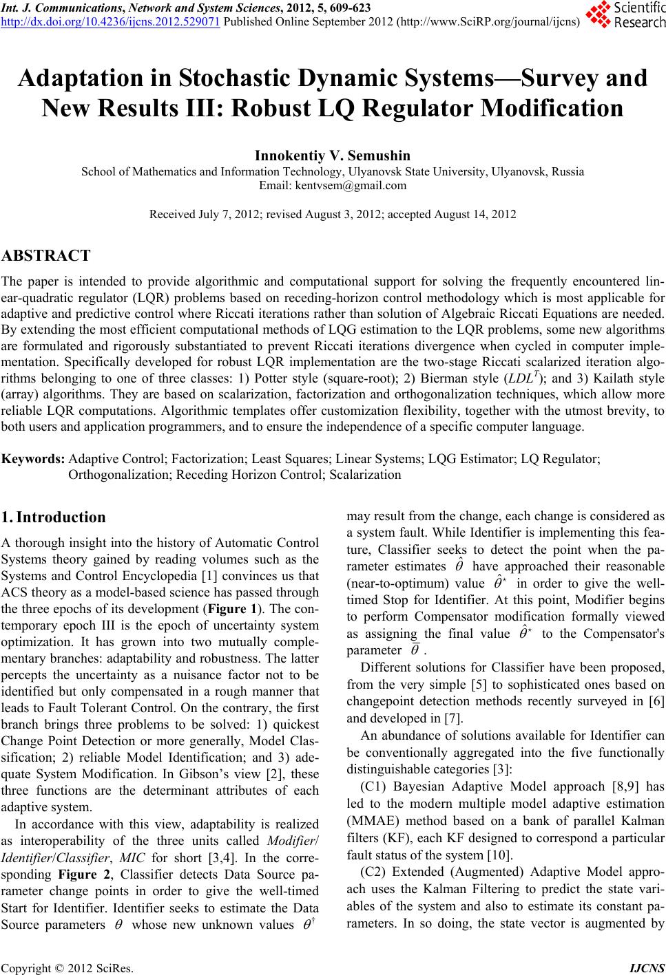
 Int. J. Communications, Network and System Sciences, 2012, 5, 609-623 http://dx.doi.org/10.4236/ijcns.2012.529071 Published Online September 2012 (http://www.SciRP.org/journal/ijcns) Adaptation in Stochastic Dynamic Systems—Survey and New Results III: Robust LQ Regulator Modification Innokentiy V. Semushin School of Mathematics and Information Technology, Ulyanovsk State University, Ulyanovsk, Russia Email: kentvsem@gmail.com Received July 7, 2012; revised August 3, 2012; accepted August 14, 2012 ABSTRACT The paper is intended to provide algorithmic and computational support for solving the frequently encountered lin- ear-quadratic regulator (LQR) problems based on receding-horizon control methodology which is most applicable for adaptive and predictive con trol where Riccati iterations rather than solution of Algebraic Riccati Equations are needed. By extending the most efficient computational methods of LQG estimation to the LQR problems, some new algorithms are formulated and rigorously substantiated to prevent Riccati iterations divergence when cycled in computer imple- mentation. Specifically developed for robust LQR implementation are the two-stage Riccati scalarized iteration algo- rithms belonging to one of three classes: 1) Potter style (square-root); 2) Bierman style (LDLT); and 3) Kailath style (array) algorithms. They are based on scalarization, factorization and orthogonalization techniques, which allow more reliable LQR computations. Algorithmic templates offer customization flexibility, together with the utmost brevity, to both users and application programmers, and to ensure the independence of a specific computer language. Keywords: Adaptive Control; Factorization; Least Squares; Linear Systems; LQG Estimator; LQ Regulator; Orthogonalization; Receding Horizon Control; Scalarization 1. Introduction A thorough insight into the history of Automatic Control Systems theory gained by reading volumes such as the Systems and Control Encyclopedia [1] convinces us that ACS theory as a model-b ased science has passed through the three epochs of its development (Figure 1). The con- temporary epoch III is the epoch of uncertainty system optimization. It has grown into two mutually comple- mentary branches: adap tability and robustness. The latter percepts the uncertainty as a nuisance factor not to be identified but only compensated in a rough manner that leads to Fault Tolerant Control. On the con trary, the first branch brings three problems to be solved: 1) quickest Change Point Detection or more generally, Model Clas- sification; 2) reliable Model Identification; and 3) ade- quate System Modification. In Gibson’s view [2], these three functions are the determinant attributes of each adaptive system. In accordance with this view, adaptability is realized as interoperability of the three units called Modifier/ Identifier/Classifier, MIC for short [3,4]. In the corre- sponding Figure 2, Classifier detects Data Source pa- rameter change points in order to give the well-timed Start for Identifier. Identifier seeks to estimate the Data Source parameters whose new unknown values † may result from the change, each change is considered as a system fault. While Identifier is implementing this fea- ture, Classifier seeks to detect the point when the pa- rameter estimates ˆ have approached their reasonable (near-to-optimum) value ˆ ˆ in order to give the well- timed Stop for Identifier. At this point, Modifier begins to perform Compensator modification formally viewed as assigning the final value to the Compensator's parameter . Different solutions for Classifier have been proposed, from the very simple [5] to sophisticated ones based on changepoint detection methods recently surveyed in [6] and developed in [7]. An abundance of solutions available for Identifier can be conventionally aggregated into the five functionally distinguishable categories [3]: (C1) Bayesian Adaptive Model approach [8,9] has led to the modern multiple model adaptive estimation (MMAE) method based on a bank of parallel Kalman filters (KF), each KF designed to correspond a particular fault status of the system [10]. (C2) Extended (Augmented) Adaptive Model appro- ach uses the Kalman Filtering to predict the state vari- ables of the system and also to estimate its constant pa- rameters. In so doing, the state vector is augmented by C opyright © 2012 SciRes. IJCNS 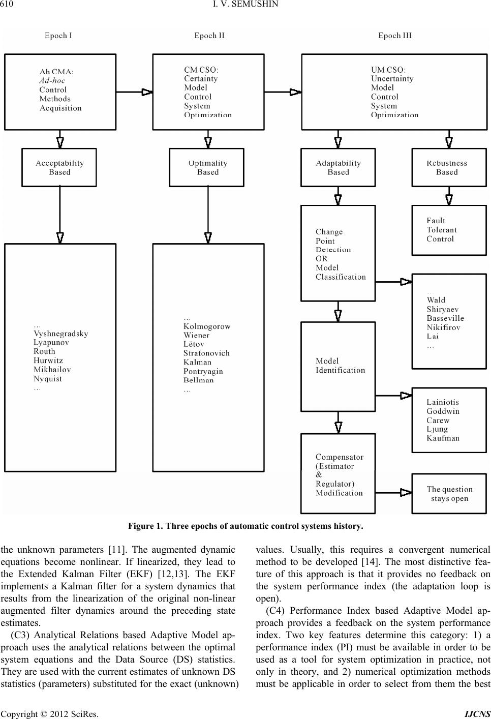 I. V. SEMUSHIN 610 Figure 1. Three epochs of automatic control systems history. the unknown parameters [11]. The augmented dynamic equations become nonlinear. If linearized, they lead to the Extended Kalman Filter (EKF) [12,13]. The EKF implements a Kalman filter for a system dynamics that results from the linearization of the original non-linear augmented filter dynamics around the preceding state estimates. (C3) Analytical Relations based Adaptive Model ap- proach uses the analytical relations between the optimal system equations and the Data Source (DS) statistics. They are used with the current estimates of unknown DS statistics (parameters) substituted for the exact (unk nown) values. Usually, this requires a convergent numerical method to be developed [14]. The most distinctive fea- ture of this approach is that it provides no feedback on the system performance index (the adaptation loop is open). (C4) Performance Index based Adaptive Model ap- proach provides a feedback on the system performance index. Two key features determine this category: 1) a performance index (PI) must be available in order to be used as a tool for system optimization in practice, not only in theory, and 2) numerical optimization methods must be applicable in order to select from them the best Copyright © 2012 SciRes. IJCNS  I. V. SEMUSHIN 611 wv Data Source † † † M Compensator ˆ : odifier ˆ ˆ ˆ Start Stop uy /Identifier Classifier Figure 2. Adaptive stochastic control system structure: stands for Plant; for Sensor; for Regulator; for Estimator. M one as the system parameters estimator able to minimize the adopted PI. They are the focus of particularly intense scrutiny, and among them most theoretically substanti- ated and practically developed is Ljungian Minimum Prediction Error (MPE) method [15,16]. A less known method belonging to the same category is the Auxiliary Performance Index (API) method which renders possible least squares fitting the adaptive model state to the pure albeit hidden DS state, not to the measured (incomplete and noisy) output [3,4]. (C5) Characteristic Matching Adaptive Model approa- ch is usually based on introdu cing into model equation s a fictitious noise with its root-mean-square (RMS) adjust- able [17,18] for a better fitting of the model. This ap- proach is adjacent to robust system control [19]. The above generalized categories are not necessarily pure, i.e. they can be met in combinations as it is the case of (C2) + (C5) in [20] or (C1) + (C2) in [21]. More to it, the same five categories hold for Classifier solutions, e.g. [22-24]. Given Classifier running as a “hot-line alert system”, a next successive adaptation period can emerge spontane- ously as a model identification phase followed by a com- pensator (Estimator & Regulator) modification phase (cf. Figures 1 and 2). For the basic Figure 2, it is claimed that in automatic control, a regulator is a device which has the function of maintaining a designated characteris- tic of the plant behaviour by transforming the estimates of plant internal states into the control inputs applied (through an actuator) to the plant. A state estimator is typically a computer-implemented mathematical model that models a real system composed of the plant and a sensor in order to provide an estimate of plant’s internal state, given measurements of the input and output of the real system, which is called Data Sourc e in Figure 2. The present paper in intended to provide algorithmic and computational perspective for answering questions on how to perform Regulator Modification phase in adaptive control systems (the lower right side block in Figure 1). It is absolutely understandable that this phase should be based on the regulator design methods, so that the very regulator modification can be treated as a re-design procedure. In this respect, we restrict ourselves to the case of discrete LQG control problem, that is, the control problem with Linear discrete-time plant and sen- sor models, and Quadratic performance index, and Gaus- sian random disturbances. Fundamental to the discrete LQG control problem are Copyright © 2012 SciRes. IJCNS  I. V. SEMUSHIN 612 tw o matrix non linear Riccati Difference Equations (RDE), which are dual to each other. The forward RDE is used in the synthesis of LQG-es- timator (LQGE, that is, Kalman Filter, KF), and the backward RDE for the design of Linear-Quadratic Regu- lator (LQR). KF and LQR are designed independently of each other (the separation principle [25]). The latter is cascaded with the first, thus closing the feedback loop (the compesa tor in Figure 2). LQR for the LQG-control law is identical to its counterpart for the LQ deterministic control law (the certainty-equivalence principle, [26], p. 228). Textbooks on LQG-control contain these well-known theoretical facts. However, not every one covers the computational aspects of RDE. Often, classic textbooks confine themselves to giving references about care or dare functions of MATLAB® [27,28] thus meaning algebraic Riccati equations (ARE) [29] which can be either continuous-time ARE (care), or discrete-time ARE (dare). Solution of ARE is the critical task for stabilizing the compensator design. For discrete-time systems, the solution to DARE coincides with the steady- state solution of the RDE approached as the control ho- rizon tends to infinity [30]. Generalized Riccati theo ry is the key tool to robust control [31]. Many textbooks on Automatic Control Systems con- tain sometimes not only the presentation or derivation of RDE, but also a summary of numerical solutions of ARE as well. For example, [32] says (Section 11.5) that cita- tion of published works on solutions and features of ARE (as of 1986) may amount to a book of its own. It men- tions an iterative method and considers, in some more detail, the iterative solution and eigenvalue methods as well. However, the main source of information on Riccati equations is the vast research literature [33]. Great atten- tion paid to ARE arises from the fact that the direct RDE iterations, even if they are taken in the robustified form (Joseph style), do not exhibit fast convergence to the steady-state positive-definite solution. The study and development of computational methods for ARE have evolved vigorously for many years. Of the great many publications, we mention only a few: [34-37] for the LQ-regulator solution and [38-44] for the LQG- estimator design. Based on these methods, solvers for ARE have been implemented in such software packages as Maple [45], Mathematica [46], MATLAB [47-49] and in computer libraries as BLAS (level I-III), EISPACK and LINPACK, as well as in their successor LAPACK [50,51]. Many Riccati solvers are written in FORTRAN, and also in Python [52]. The number of publications on ARE solvers has continued to grow [53-55]. Efficient use of existing methods within the software packages and libraries is mostly meant for off line appli- cations owing to their high comptutational cost. For in- stance, at each Kleinmann iteration step [56], the com- putationally expensive Lyapunov equation has to be solved ([26], pp . 34-121) . Newton ’s method [ 57] r equir es solving a Lyapunov equation in the main step ([54], p. 6). Schur method [34], the most popular one amongst the eigenvalue methods, also needs considerable computa- tion efforts and additional details to make this approach work satisfactorily. All these methods are intended for solving ARE, and so their ultimate end is to find a stabilizable regulator solution [58]. However, sometimes there is no need for solving ARE. Such a category of problems includes the Model Predictive Control, or MPC [26,59] ex ploiting the idea of finite receding horizon control (RHC) [26]. In finite RHC, the attainment of the steady-state Riccati solution is not the case due to the very sense of words “finite horizon” and “system adaptation” as can be seen from the generalized adaptive stochastic control system structure (in Figure 2, reproduced from [4]). This ex- plains why we do not consider the above surveyed methods of solving ARE advisable for regulator modifi- cation (re-design) in the adaptive control structure of Figure 2. In this paper, we consider the duality relations between the two RDE, that are at the heart of LQGE on the one part, and LQR on the other part, to secure further ad- vancement in the algorithms for Linear-Quadratic Regu- lator Optimization [51]. In doing so, we expect the com- putational methods, which have been derived for the LQG-Estimator implementation over the preceding dec- ades and recently surveyed in [60], to be successfully extended to the LQR re-design where a stepwise solution for the (backward) RDE, rather than ARE, is of primary importance. In Section 2 we formulate Problem 1 of determining the LQG control law for the system composed of the plant and sensor both linearly modeled and subjected to additive Gaussian wh ite noises [26,61]. Section 3 describes Problem 2 of LQG receding hori- zon control in line with [26]. Solutions to the above two problems are presented in Section 4 in order to compare both forward and back- ward RDEs and then to move to a single Riccati iteration (aiming at the backward RDE) which is given in Section 5 in an intermediate abstract notation. In Section 6, we split the single Riccati iteration into two consequtive stages in order to construct two separate computational procedures called “Riciup Riccati Instant Update” and “Rictup Riccati Temporal Up- date,” which we use as the starting point for their nu- merical robustification. Section 7 presents the scalarization of Riciup. By this equivalent transformation, we have prepared both Copyright © 2012 SciRes. IJCNS  I. V. SEMUSHIN 613 stages for the three robust modification styles: Potter style in Section 8, Bierman style in Section 9 an d Kailath style in Section 10. Section 11 provides a brief look at the typical applica- tions of the results discussed in this paper, together with a characterization of related challenges. The paper closes with the concluding remarks about the novelty of the new algorithmic insights. 2. LQG Control Problem The overall system model includes: an n-dimentional stochastic discrete-time plant state equation 11 00 , 0,1, ;, i iii 0 , ii i tttxtB ixtx tutwt P (1) and a m-dimentional measurement (sensor) equation ,1,2,, i i iii ytHtxtvt (2) where 01 ,,wt vt >0 i Rt wt 0 and 12 are two mutually independent noise sequences of independent Gaussian (normal) zero mean random vectors represent- ing the state disturbance w and the measurement error v, characterized by covariance matrices i (posi- tive semi-definite) and (positive definite) cor- respondingly and independent of Gaussian initial state ,,vt 0Qt t of mean 0 and covariance matrix . Control 0 P 0 N kk uut ,,,t ut input is assumed to be sought as a 0,N sequence N of r-dimentional con- trol vectors which are applied to (1) to minimize the mean square performance index, PI (the expected cost) on a finite horizon of N time steps: 01 ut u k ut 00 0, 22 0 ,, kk N N kk tt k Jt xtu Ext ut 2 1. f N xt (3) where the equivalence symbol reads “is equal by defini- tion to”. It is assumed that any nonzero input ut k within the prediction horizon incurres a cost. This am- ounts to assuming that each weighting matrix k t 0 T tt t , which is symmetric, is positive definite (PD): kk . Further, it is assumed that the in- stantaneous cost at time k (the term within parentheses in (3)) is nonnegative. Together with the above PD con- dition, this is equivalent to the semi-positive definiteness of each symmetric matrix : T kk tt 0 k t. The terminal (or final) cost 2 1 N 0 xt is also assumed nonnegative, hence (f T ff inal ). Remark 1. Expectation operator E in (3) is de- fined w.r.t. probability measures induced by 000 , txP 0, ii wt Qt, and 0,vt Rt ii Remark 2. Metric in (3) is chosen to be elliptic: . 2 k T kkkk t txttxt and so on. By means of it, one can regulate the impor- tance of any summand in criterion (3). For example, the more costly is a single (the j-th) control input k ut 0kN within the prediction control horizon (PCH, k t ), the greater should be its weight defined as the j-th di- agonal element of matrix in comparison with others. tk, tk, Selecting N t as identity matrices brings us back to classical spherical distance measures. In signal processing, one needs sometimes to emphasize specific directions/dimentional components where statis- tical facts are more relevant. This is called ICA (Inde- pendent Component Analysis) [62]. Remark 3. The length of PCH, N in (3), approaching infinity () is not a judicious choice for adaptive systems. Infinitely large N would mean the intention to attain a steady-state mode of cont rol, when no unforeseen model changes are considered anymore. This is in deep contradiction with the very sense of adaptation. Thus, N must be finite. A question arises: what finite value of N can be selected? Obviously, it depends on the mechanism which the unforeseen changes are subject to. By assump- tion, these changes should not occur very frequently compared with the control system transition time in order let the adaptor keep up with the dynamics of changes. If the changes mechanism operates as an independent actor, it is reasonable to take N equal or greater than the ex- pected time interval between the neighbouring model change points. Remark 4. Weighting matrices k and tk can be time-dependent within the PCH. There are many ways to do so. A reasonable one would be a matrix or- dering: both weighting matrix sequences are chosen in decreasing order (Version 1) 01 01 N N tt t tt t (4) or in increasing order (Version 2) 01 01 N tt t tt t 1 tt (5) where the matrix inequality is interpreted as the standard positive matrix inequality: 0, meaning 0tt 01 and so on. Remark 5. In adaptive systems, our knowledge of how the matrices describing models (1), (2) behave is getting more and more vague in course of time within the Copyright © 2012 SciRes. IJCNS  I. V. SEMUSHIN 614 PCH. Common sense seems to tell us that this fact gives us reasons for prefering the decreasing version (4). In this case, the instantaneous cost at a farther time tk as part of penalty criterion (3), will be less than at preceding times. Working with decreasing sequences (4) can be also justified on grounds of RHC. As described in Sec- tion 3, all the control inputs except for the first one, which are found to minimize the overal RHC cost, are discarded anyway. On the other hand, the choice of (4) can mean under- estimating the risk of farther erroneous states k t ut 0t 0 f 0, = and wrong controls k caused just by our vague knowl- edge of how the matrices describing models (1), (2) will behave in future. To mitigate the risk, one should prefer the increasing version (5). Thus, it becomes clear that the cost behaviour of con- trol, especially of RHC, is a serious issue deserving a special study and experimenting which is planned to be made beyond the scope of this paper. The standard LQG control problem (P1) is stated as follows. Problem P1 Consider (1) and (2) as the linear models of a plant and a sensor subject to Gaussian excitations w and v. Define the quadratic performance index (3) with the symmetric matrices , k and . Find an optimal physically feasible control input >0 k t uu to the plant (1), initialized from the event 00 ,txt ut , minimizing the performance index (3). Remark 6. The notion “physically feasible” applied to control inputs here and below infers cause-and-effect relationships between control inputs i and system outputs i yt i t : the first can not appear before the lat- ter. 3. Receding Horizon (LQG) Control RHC was introduced by French engineer Richalet and his colleagues in 1978 [59] to relax the computational diffi- culties of steady-state control [26]. In the LQG frame- work, the RHC problem (P2) looks as follows. Problem P2 Consider (1) and (2) as the linear models of a plant and a sensor subject to Gaussian noise inputs w and v. RHC Procedure: At time , define the quadratic PI , 22 = ,, kk ii ii N iN kk tt ki Jtxt u Ext ut 2 1f iN xt 0 (6) for s ymmetri c matr ices , > k t 0 k t and f0 t , iN ut . At , find an optimal physically feasible sequence i 1 ,,, ii ii N uutut starting with the event ,txt ii , minimizing the performance index (6). Apply to the plant (1) the initial control vector ut 1i t i of the optimal sequence whose subsequent N vectors are discarded. Repeat the procedure at time to select 1i ut from the next optimal sequence 12 1 1, 1,,, ii iN ii N uututut ,txt tt t . Although so defined RH LQG control can be hardly considered “optimal” in a rigor sense, it has attractive features [26] thus prompting suggestions that the RHC be used as the basis in the adaptive control structure (of Figure 2) for robust regulator computations as done in the sections that follow. 4. Riccati-Based Solution From the comparison of P1 and P2 statements, in order to obtain criterion (6) from criterion (3) one should ad- vance the (zero-indexed) event 00 , which is ini- tial for the whole control sequence in P1, i steps: 00ii, and so 0,0, , iiN iiN uu . There- fore all the subsequent results concerning regulation problems will be formulated for P1. They can be shifted in parallel i steps ahead to obtain the corresponding cor- rect result for P2. u 0,1, ,iN Theorem 1 [26]. Optimal LQG-control law is decom- posed into two independent series-connected parts 4.1 and 4.2: 4.1. Optimal (Kalman) Filter, KF Equations 1) For the KF computes the extrapo- lated estimates ˆ1i t for 1i t i t1i . They are obtained through the temporal update, from to t, of the fil- tered estimates ˆi as t 11 ˆˆ , iiiiii tttxtBtut (7) with 00 0 ˆ:xtx Ext and the covariance matri- ces 111 ,, T iiiiiii tQtttPttt where 0 00000 :T PtPE xtxxtx . 1, 2,,iN 2) For the KF computes the so-called filtered (that is measurement updated) estimates ˆi t . They are obtained through the measurement update using ii zzt >0 i Rt i with covariances at t, as ˆˆˆ iifiiii txtKtzHtxt filt er f (8) ) with the filter gain ( 1 TT fiiiii ii KtPtHtRtHt Pt Ht and also the filtered estimates covariance matrices Copyright © 2012 SciRes. IJCNS 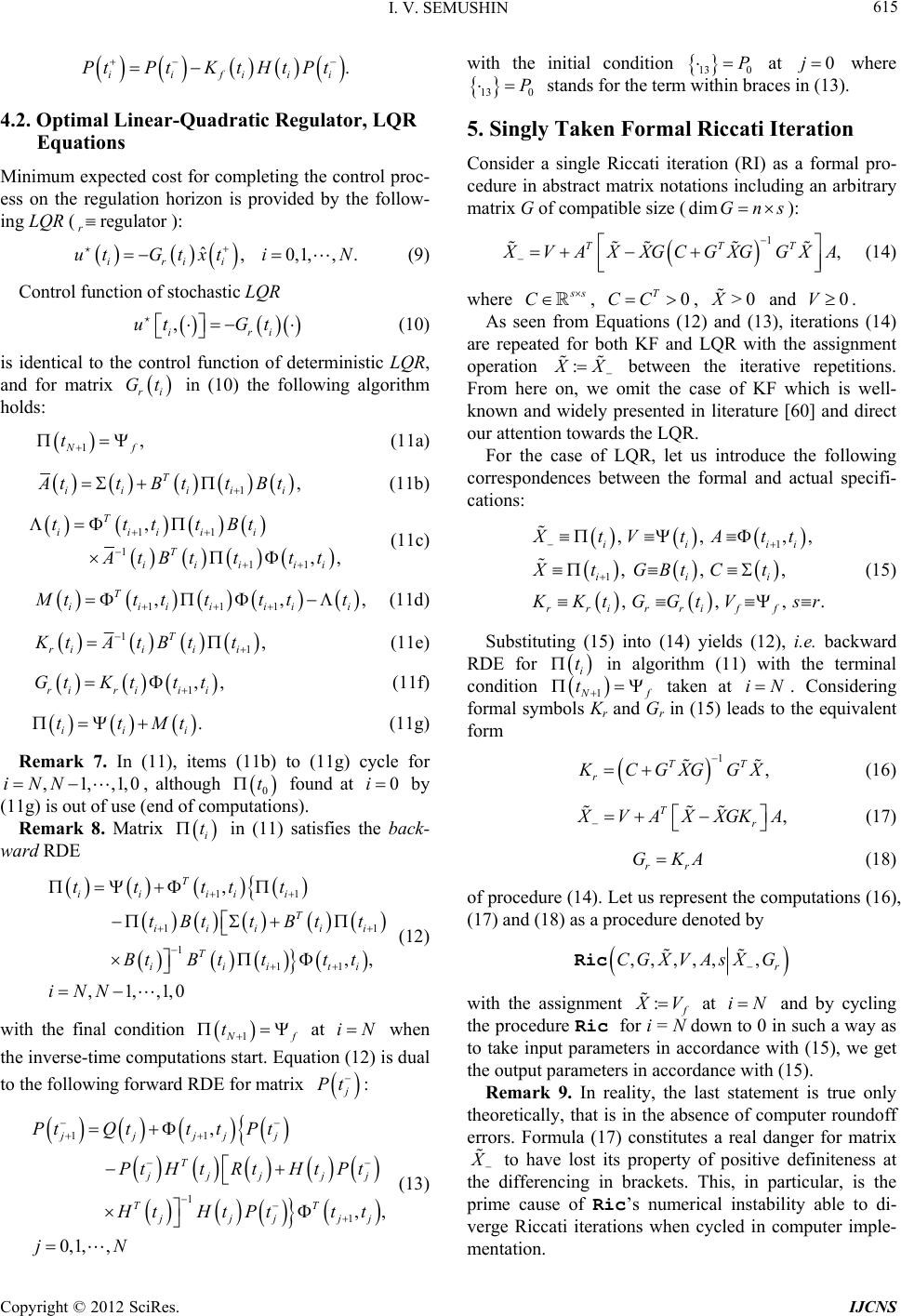 I. V. SEMUSHIN 615 iii . iif tPtK tHtPt regulat o r r ,0 ,1,,.i N , iri ut Gt ri Gt 1, 4.2. Optimal Linear-Quadratic Regulator, LQR Equations Minimum expected cost for completing the control proc- ess on the regulation horizon is provided by the follow- ing LQR (): ˆ irii ut Gtxt (9) Control function of stochastic LQR (10) is identical to the control function of deterministic LQR, and for matrix in (10) the following algorithm holds: f t (11a) 1, T ii iii ttBttBt (11b) 1 11 11 ,, ii T iiiii tBt, T iii ttt tB tttt 111 ,,, T iiiiiii (11c) ttttttt (11d) 11, T riii i KtA tBtt (11e) 1, i i t t iii Mt ,,1,0 0 t0i , (11f) ri ri Gt Kt tt. (11g) Remark 7. In (11), items (11b) to (11g) cycle for , although found at ,1iNN by (11g) is out of use (end of com putations). Remark 8. Matrix i t in (11) satisfies the back- ward RDE 11 11 11 , ,, T ii iii T iii ii iti t t tBtt Btt t t 1 ,1 ,,1,0 T ii BtB tt iNN 1 tt t (12) with the final condition f N t at i when the inverse-time computations start. Equation (12) is dual to the following forward RDE for matrix t : jj T jj jj 11 1 , ,, j j jj T 1 0, 1,, T jj jj Pt Ht Pt Qt t PtH t Pt Rtt tHtPt jN tt P 0j (13) with the initial condition 130 at where 13 0 P Gn s 1, TTT stands for the term within braces in (13). 5. Singly Taken Formal Riccati Iteration Consider a single Riccati iteration (RI) as a formal pro- cedure in abstract matrix notations including an arbitrary matrix G of compatible size (dim ): VAXXGCGXGGXA (14) s C 0 T CC, where >0X 0 : , and V. As seen from Equations (12) and (13), iterations (14) are repeated for both KF and LQR with the assignment operation X between the iterative repetitions. From here on, we omit the case of KF which is well- known and widely presented in literature [60] and direct our attention towards the LQR. For the case of LQR, let us introduce the following correspondences between the formal and actual specifi- cations: 1 1 ,,,, ,,, ,,,. iiii iii rrirriff XtVtAtt XtGBtCt KtG GtVsr (15) Substituting (15) into (14) yields (12), i.e. backward RDE for i t in algorithm (11) with the terminal condition 1 f t iN 1, TT r taken at . Considering formal symbols Kr and Gr in (15) leads to the equivalent form CGXG GX , Tr (16) VAXXGKA rr GKA (17) (18) of procedure (14). Let us represent the computations (16), (17) and (18) as a procedu re d enoted by ,,,,,,r CGXVAsXG Ric : with the assignment V N at i and by cycling the procedure Ric for i = N down to 0 in such a way as to take input parameters in accordance with (15), we get the output parameters in accordance with (15). Remark 9. In reality, the last statement is true only theoretically, that is in the absence of computer roundoff errors. Formula (17) constitutes a real danger for matrix to have lost its property of positive definiteness at the differencing in brackets. This, in particular, is the prime cause of Ric’s numerical instability able to di- verge Riccati iterations when cycled in computer imple- mentation. Copyright © 2012 SciRes. IJCNS 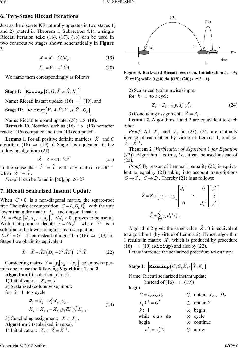 I. V. SEMUSHIN 616 6. Two-Stage Riccati Iterations Just as the discrete KF naturally operates in two stages 1) and 2) (stated in Theorem 1, Subsection 4.1), a single Riccati iteration Ric (16), (17), (18) can be used in two consecutive stages shown schematically in Figure 3 ˆ, r XXGK ˆ. T (19) VAXA (20) We name them correspondingly as follows: Stage I: ˆ , ,r CGXsXK ,, Riciup Name: Riccati instant update: (16) (19), and Stage II: ˆ, , rr XK sXG Rictup ,, , VA Name: Riccati temporal update: (20) (18). Remark 10. Notation such as (16) (19) hereafter reads: “(16) computed and th en (19) com put ed”. Lemma 1. For all positive definite matrices nd C algorithm (16) 19) of Stage I is equivalent to the following algorithm (21) a ( 1 ˆT ZGCG 1 ˆˆ (21) in the sense that Xns G with any matrix when 1 X . Proof. It can be found in [40], pp. 26-27. 7. Riccati Scalarized Instant Update When is a non-diagonal matrix, the square-root free Cholesky decomposition CC C with the unit lower triangular matrix C and diagonal matrix >0CT CLDL L 12 ,,,dd Cs , , proves to be useful. With that purpose denote C YG , where Y is a solution to the lower triangular matrix equation C. Then instead of algorithm (16) (19) for Stage I we obtain its equivalent Dd g T G dia >0 k dT L T ˆ. TT T LY 1 C XXYDYXY YX (22) Considering matrix 12 Yyy y : columnwise per- mits one to use the following Algorithms 1 and 2. Algorithm 1 (scalarized, direct). 1) Initialization: 0 X. 2) Scalarized (columnwise) input: for to s cycle 1k 1 11 kk kk kk XX X 11 , . Tk T kkkkk dyXy y yX ˆ: (23) 3) Concluding assignment: X 1 . Algorithm 2 (scalarized, inverse). 1) Initialization: 0: ZX X ˆ XX 1i ti ttime (20) (19) . Figure 3. Backward Riccati recursion. Initialization i := N; := Vf; while (i ≥ 0) do {(19); (20); i := i − 1}. 2) Scalarized (columnwise) input: 1k to s cycle for 1 1. T kk kkk Zydy ˆ: (24) Z 3) Concluding assignment: . Lemma 2. Algorithms 1 and 2 are equivalent to each other. Proof. All k and k in (23), (24) are mutually inverse of each other by virtue of Lemma 1, and so, 1 ˆˆ X . Theorem 2 (Verification of Algorithm 1 for Equation (22)). Algorithm 1 is true, i.e., it can be used instead of (22). Proof. By reason of Lemma 1, equality (22) is equiva- lent to equality (21) taking into account transcriptions , . Thereby (21) is as follows: GYCD 1 11 11 1 1 0 ˆ 0 . T sT s sT kk k k dy ZZ yy dy Zydy ˆ Algorithm 2 gives the same value . It is equivalent to algorithm 1 (by virtue of Lemma 2). Hence, algorithm 1 results in matrix ˆ , which is produced by procedure (16) (19) (Riciup) and also by (22). Let us introduce the scalarized procedure Ricsiup: Stage I: ˆ ,,, ,r CGXsXK Ricsiup T CCC CLDLC LC D TT C LY G :1k Name: Riccati scalarized instant update (instead of (16) (19)) begin obtain , obtain Y begin ks while do cycle : TT k pyX begin continue a row Copyright © 2012 SciRes. IJCNS 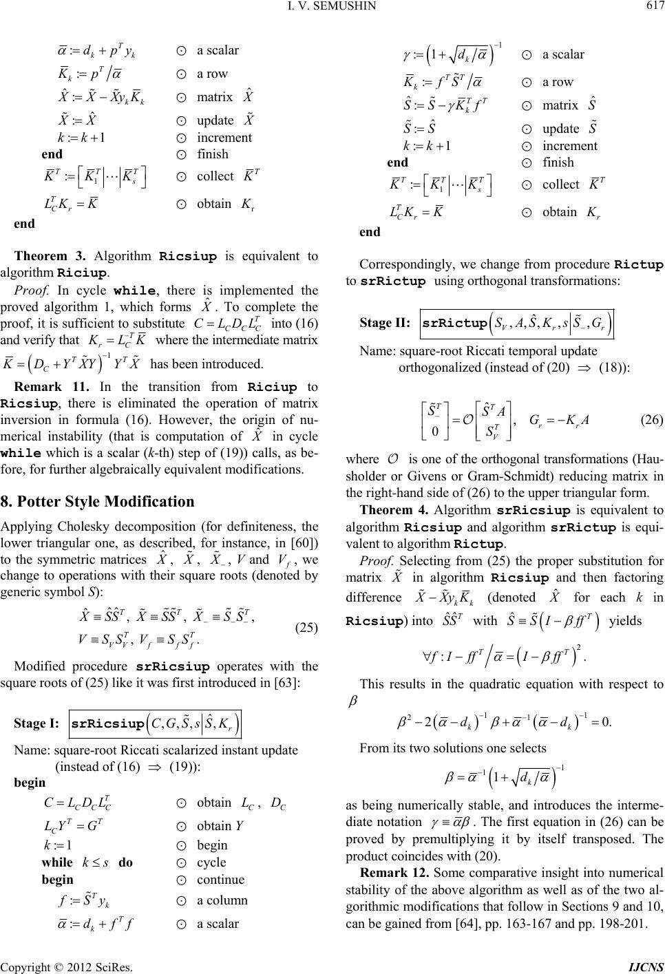 I. V. SEMUSHIN 617 :T kk y dp a scalar : k Kp T a row ˆ:kk XX yK ˆ matrix ˆ : X update kk :1 increment end finish 1 TT :T KK collect T T Cr LK r K obtain end Theorem 3. Algorithm Ricsiup is equivalent to algorithm Riciup. Proof. In cycle while, there is implemented the proved algorithm 1, which forms ˆ . To complete the proof, it is sufficient to substitute CC C into (16) and verify that T CLDL T Cr L K where the inter mediate matrix C 1 TT DYXYYX ˆ has been introduced. Remark 11. In the transition from Riciup to Ricsiup, there is eliminated the operation of matrix inversion in formula (16). However, the origin of nu- merical instability (that is computation of in cycle while which is a scalar (k-th) step of (19)) calls, as be- fore, for further algebraically equivalent modifications . 8. Potter Style Modification Applying Cholesky decomposition (for definiteness, the lower triangular one, as described, for instance, in [60]) to the symmetric matrices ˆ , , , V and V , ,. T TT f , we change to operations with their square roots (denoted by generic symbol S): ˆˆ ˆ,, TT VV ff SSX SS VSSVS XSS S (25) Modified procedure srRicsiup operates with the square roots of (25) like it was first introduced in [63]: Stage I: ˆ ,,, ,r SsSK CC CLC LC D T C LY :1 k : CGsrRicsiup Name: square-root Riccati scalarized instant update (instead of (16) (19)): begin T C DL obtain , T G obtain Y begin while do cycle ks begin continue Tk Sy a column :Tf k df a scalar 1 :1 k d a scalar :TT k KfS a row ˆ:TT k SS Kf ˆ S ˆ :SS matrix S :1kk update increment end finish 1 : TTT KK collect T T Cr LK K obtain r end Correspondingly, we change from procedure Rictup to srRictup using orthogonal transformations: Stage II: ˆ ,,,,, Vrr SASKsSG srRictup ˆ, 0 TT rr T V SSAGKA S Name: square-root Riccati temporal update orthogonalized (instead of (20) (18)): (26) where is one of the orthogonal transformations (Hau- sholder or Givens or Gram-Schmidt) reducing matrix in the right-hand side of (26) to the upper triangular form. Theorem 4. Algorithm srRicsiup is equivalent to algorithm Ricsiup and algorithm srRictup is equi- valent to algorithm Rictup. Proof. Selecting from (25) the proper substitution for matrix in algorithm Ricsiup and then factoring difference kk Xy K ˆ (denoted for each k in Ricsiup) into with SS yields ˆˆT SS ˆT I ff 2 :. TT fI ffIff This results in the quadratic equation with respect to 11 21 20. kk dd From its two solutions one selects 1 11k d as being numerically stable, and introduces the interme- diate notation . The first equation in (26) can be proved by premultiplying it by itself transposed. The product coincides with (20). Remark 12. Some comparative insight into numerical stability of the above algorithm as well as of the two al- gorithmic modifications that follow in Sections 9 and 10, can be gained from [64] , pp. 163-167 and pp. 198-201. Copyright © 2012 SciRes. IJCNS 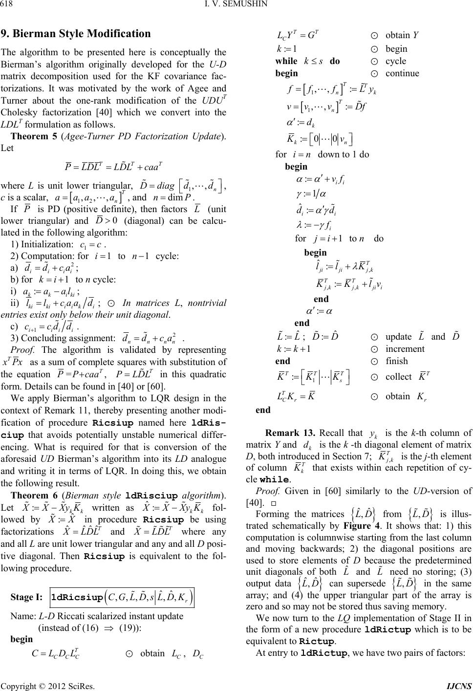 I. V. SEMUSHIN 618 9. Bierman Style Modification The algorithm to be presented here is conceptually the Bierman’s algorithm originally developed for the U-D matrix decomposition used for the KF covariance fac- torizations. It was motivated by the work of Agee and Turner about the one-rank modification of the UDUT Cholesky factorization [40] which we convert into the LDLT formulation as follows. Theorem 5 (Agee-Turner PD Factorization Update). Let TTT LDL caa 1,, n Ddd diag aadimnP PLDL where L is unit lower triangular, , c is a scalar, , and . 12 ,,, T n a a If P is PD (positive definite), then factors L (unit lower triangular) and 0D (diagonal) can be calcu- lated in the following algorithm: 1) Initialization: . 1 2) Computation: for to cycle: cc1i1n a) 2 ii a ii b) for to n cycle: dd c 1ki : kkiki aaal ; i) ; ii) kikiiiki ; In matrices L, nontrivial entries exist only below their unit diagonal. llcaad c) 1iiii 3) Concluding assignment: ccdd . 2 ddca nn nn Proof. The algorithm is validated by representing . T Px as a sum of complete squares with substitution of the equation =, T PPcaaT PLDL in this quadratic form. Details can be found in [40] or [60]. We apply Bierman’s algorithm to LQR design in the context of Remark 11, thereby presenting another modi- fication of procedure Ricsiup named here ldRis- ciup that avoids potentially unstable numerical differ- encing. What is required for that is conversion of the aforesaid UD Bierman’s algorithm into its LD analogue and writing it in terms of LQR. In doing this, we obtain the following result. Theorem 6 (Bierman style ldRisciup algorithm). Let :kk XXyK written as ˆ:kk XXyK ˆ : fol- lowed by X in procedure Ricsiup be using factorizations ˆˆˆˆ T LDLT and LDL where any and all L are unit lower triangular and any and all D posi- tive diagonal. Then Ricsiup is equivalent to the fol- lowing procedure. Stage I: ˆˆ ,, ,,r DsLDK T CCC CLDLC LC D TT C LY G :1k ,, CGL 1dRicsiup Name: L-D Riccati scalarized instant update (instead of (16) (19)): begin obtain , obtain Y begin kswhile do cycle 1,,: TT nk begin continue ff Ly 1,, : T n vv vDf :k d :0 0 kn v in for down to 1 do begin :ii vf :1 ˆ: ii dd :i f 1ji to n do for begin , ˆ:T ijijk ll K ,, : TT kjkjii Klv : end end ˆ : LL ˆ : DD; L D :1kk update and increment end finish 1 : TTT KK collect T T Cr LK K obtain r end Remark 13. Recall that k is the k-th column of matrix Y and k is the k -th diagonal element of matrix D, both introduced in Section 7; y d , T k is the j-th element of column T k that exists within each repetition of cy- cle while. Proof. Given in [60] similarly to the UD-version of [40]. Forming the matrices ˆˆ , LD ,LD ˆ L L from is illus- trated schematically by Figure 4. It shows that: 1) this computation is columnwise starting from the last column and moving backwards; 2) the diagonal positions are used to store elements of D because the predetermined unit diagonals of both and need no storing; (3) output data ˆˆ , LD ,LD can supersede in the same array; and (4) the upper triangular part of the array is zero and so may not be stored thus saving memory. We now turn to the LQ implementation of Stage II in the form of a new procedure ldRictup which is to be equivalent to Rictup. At entry to ldRictup, we have two pairs of factors: Copyright © 2012 SciRes. IJCNS 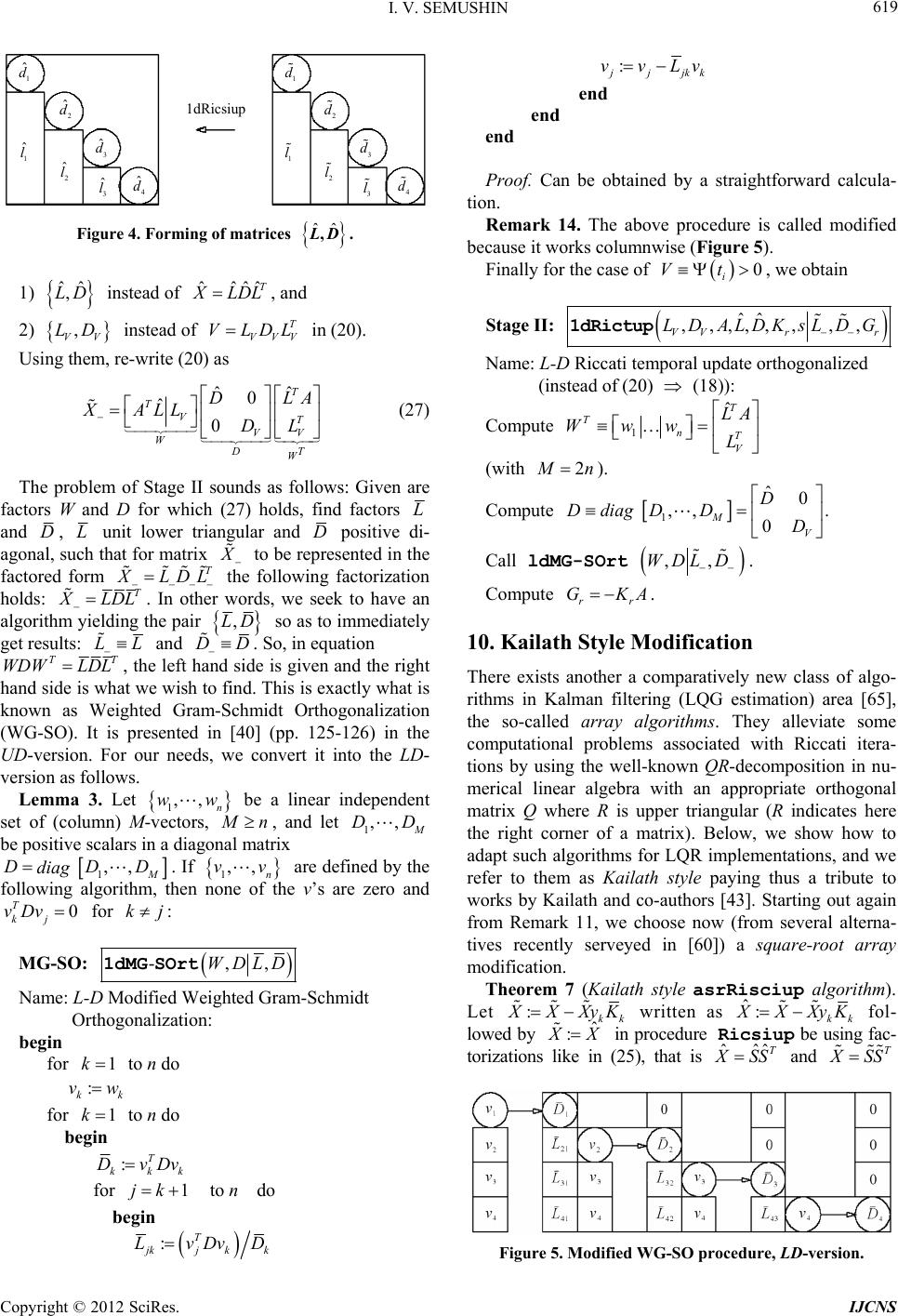 I. V. SEMUSHIN 619 1 ˆ d 2 ˆ d 3 ˆ d 4 ˆ d 1 d 1 ˆ l 2 ˆ l 3 ˆ l 1 l 1dRicsiup 2 d 3 d 4 d 2 l 3 l Figure 4. Forming of matrices ˆˆ ,LD ˆ, LD ˆˆˆˆ T . 1) instead of ˆ LDL , V LD T VVV VLDL , and 2) instead of in (20). V Using them, re-write (20) as ˆˆ 0T T VV DT W DLA DL ˆ0 TV W XA LL (27) The problem of Stage II sounds as follows: Given are factors W and D for which (27) holds, find factors L and D, L unit lower triangular and D positive di- agonal, such that for matrix T to be represented in the factored form LD L the following factorization holds: T LDL . In other words, we seek to have an algorithm yielding the pair ,LD so as to immediately get results: LL and DD . So, in equation T LDL ,, n ww T WDW , the left hand side is given and the right hand side is what we wish to find. This is exactly what is known as Weighted Gram-Schmidt Orthogonalization (WG-SO). It is presented in [40] (pp. 125-126) in the UD-version. For our needs, we convert it into the LD- version as follows. Lemma 3. Let 1 be a linear independent set of (column) M-vectors, n, and let 1,, DD be positive scalars in a diagonal matrix 1M. If 1 are defined by the following algorithm, then none of the v’s are zero and for : ,,DD diag 0 kj v D j T vD ,, n vv k MG-SO: -,,WDLD 1k : kk vw 1k 1dMG SOrt Name: L-D Modified Weig hted Gram-Schmidt Orthogonalization: begin for to n do for to n do begin :T kkk DvDv 1jk for to n do begin :T kjkk LvDvD : jjkk vvLv end end end 0 i Vt Proof. Can be obtained by a straightforward calcula- tion. Remark 14. The above procedure is called modified because it works columnwise (Figure 5). Finally for the case of , we obtain ˆˆ ,,,,,, ,, VV rr LD ALDKsLDG 1dRictup Stage II: Name: L-D Riccati temporal update orthogonalized (instead of (20) (18)): Compute 1 ˆT TnT V LA WwwL 2 n(with ). Compute 1 ˆ0 ,, . 0 M V D DDD diag D Call ldMG-SOrt ,,WDL D rr GKA . Compute . 10. Kailath Style Modification There exists another a comparatively new class of algo- rithms in Kalman filtering (LQG estimation) area [65], the so-called array algorithms. They alleviate some computational problems associated with Riccati itera- tions by using the well-known QR-decomposition in nu- merical linear algebra with an appropriate orthogonal matrix Q where R is upper triangular (R indicates here the right corner of a matrix). Below, we show how to adapt such algorithms for LQR implementations, and we refer to them as Kailath style paying thus a tribute to works by Kailath and co-authors [43]. Starting out again from Remark 11, we choose now (from several alterna- tives recently serveyed in [60]) a square-root array modification. Theorem 7 (Kailath style asrRisciup algorithm). Let ˆ: :kk XXyK written as kk XXyK ˆ : fol- lowed by X ˆˆ ˆT in procedure Ricsiup be using fac- torizations like in (25), that is SS T and SS Figure 5. Modified WG-SO procedure, LD-version. Copyright © 2012 SciRes. IJCNS  I. V. SEMUSHIN 620 with both S lower triangular. Then Ricsiup is equiva- lent to the following procedure. Stage I: ˆ ,,, ,r SsSK CC CLC LC D T C LY :1k CGasrRicsiup Name: array square-root Riccati scalarized instant update (instead of (16) (19)): begin T C DL obtain , T G obtain Y begin while do cycle ks begin continue :k d : TT nk 1,, ff Sy 0 T k QfS : S S 1 : 0 k T K S (T) ˆ S update :kk increment end finish 1 TT :T KK collect T T Cr LK r K obtain end Proof. Assignment operator (T) in the above algorithm contains two arrays: pre-array B (on the right) and post-array A (on the left). At each cycle, let the latter be obtained from the first in the upper triangular form by means of an appropriate orthogomal transformation k (it may be Hausholder reflections or Givens rotations): k Q QB. Since kk QQ , we have and via straightforward calculations, we are done. TTT AAIBB Stage II in this modification coincides with Stage II in the Potter style modification, that is expression (26). 11. Applications Challenges Possible applications of adaptation capability of stochas- tic systems are numerous and can be found in almost every field of modern engineering. While considering applicability of the above results, one should select the cases that seem to fit perfectly in the pattern of Figure 2. In this pattern, the very necessity for adaptation is con- sidered as a factual constraint the occurrence of which in time is comparatively rare resulting from an abrupt fault against the long lasting nominal mode of system opera- tion. This can be exemplified by the development and implementation of a high integrity navigation system based on the combined use of an inertial measurement unit aided by different outer sources of data [20,66] some of which are fault-susceptible or working in an accident- prone situation. Famous industrial/technological study cases to be brought forward as applications to theoretical/computa- tional work are those on advanced MPC collected in [59]. Overall, we have to admit that practical problems are much more challenging than theoretical ones. One barrier to overcome is the nonlinearity of the original system (Data Source) models. The traditional remedy for this is to invoke a linearized perturbation model or equation of the first variation about a nominal (or reference) solution to the nonlinear model on the assumption that such a solution is known (as in [67 ]) or deliver ed by an External (more precise) Data Source. In the strict sense, equation (1) has been written yet in the form of perturbation model, as it can be seen from criterion (3). The latter case, combining the use of the Global Positioning System (GPS acting as an external data source) and an inertial measurement unit for vehicle applications, can be viewed as a modeling technique for online estimation of the error between the reference model and the real dynamics [68]. Another challenge to be considered is a set of con- straints representing the physical limitations of the proc- ess variables as is the case in MPC and optimization for paperma king machines [69]. 12. Concluding Remarks The emphasis in this paper has been on the robust linear quadratic regulator computations where the single Ric- cati iteration algorithm is an integral part and where seeking a steady-state Riccati solution (Algebraic Riccari Equation) does not apply. Main novelty of the results is technical: we have shown that linear algebra methods of input scalarization, matrix factorization and array orthogonalization earlier known for the robustified linear quadratic estimators due to [40, 63,65] and many other works, now are successfully ex- tended to the robust LQR computation problems includ- ing LQ Regulator Modification phase in the adaptive control systems. The new algorithmic LQ regulator for- mulations based on these methods enhance LQR numeric robustness and generate a productive perspective for fur- ther investigations into the regulator modification (re- design) methods within the structure of adaptive control. Further research is encouraged into the advancement of new insights about the numerics of LQR/ARE/DARE procedures, thus leading to Adaptive Control System CAD that is expected to include all three ACS phases— Modifier/Identifier/Classifier. 13. Acknowledgements The author would like to express his gratitude to an C opyright © 2012 SciRes. IJCNS  I. V. SEMUSHIN 621 anonymous reviewer for a number of suggestions that helped to improve the style of this paper. REFERENCES [1] M. G. Singh, “Systems and Control Encyclopedia: The- ory, Technology, Applications,” Pergamon Press, Inc., Elmsford, 1986. [2] J. E. Gibson, “Nonlinear Automatic Control: Chapter 11,” McGrow Hill, New York, 1962. [3] I. V. Semushin, “Adaptation in Stochastic Dynamic Sys- tems—Survey and New Results I,” International Journal of Communications, Network and System Sciences, Vol. 4, No. 1, 2011, pp. 17-23. doi:10.4236/ijcns.2011.41002 [4] I. V. Semushin, “Adaptation in Stochastic Dynamic Sys- tems—Survey and New Results II,” International Journal of Communications, Network and System Sciences, Vol. 4, No. 4, 2011, pp. 266-285. doi:10.4236/ijcns.2011.44032 [5] I. V. Semushin and S. A. Ponyrko, “On the Choice of Start-Stop Algorithm while Minimizing the Square Mean Performance Index,” Autometria, Siberian Division of the USSR Academy of Sciences, No. 2, 1973, pp. 68-74. [6] T. L. Lai, “Sequential Changepoint Detection in Quality Control and Dynamical Systems,” Journal of the Royal Statistical Society, Series B (Methodological), Vol. 57, No. 4, 1995, pp. 613-658. [7] T. L. Lai and H. P. Xing, “Sequential Change-Point De- tection When the Pre- and Post-Change Parameters Are Unknown,” Technical Report No. 2009-5, Department of Statistics, Stanford University, Stanford, 2009. [8] D. G. Lainiotis, “Partitioning: A Unified Framework for Adaptive Systems, I. Estimation,” Proceedings of the IEEE, Vol. 64, No. 8, 1976, pp. 1126-1143. doi:10.1109/PROC.1976.10284 [9] D. G. Lainiotis, “Partitioning: A Unified Framework for Adaptive Systems, II. Control,” Proceedings of the IEEE, Vol. 64, No. 8, 1976, pp. 1182-1197. doi:10.1109/PROC.1976.10289 [10] M. Athans and C.-B. Chang, “Adaptive Estimation and Parameter Identification Using Multiple Model Estima- tion Algorithm,” Technical Note, Lincoln Lab, MIT, Le- xington, 1976. [11] G. C. Goodwin and K. S. Sin, “Adaptive Filtering Predic- tion and Control,” Prentice Hall, Englewood Cliffs, 1984. [12] H. W. Sorenson, “Kalman Filtering: Theory and Applica- tion,” IEEE Press, New York, 1985. [13] J. K. Uhlmann, “Algorithms for Multiple Target Track- ing,” American Scientist, Vol. 80, No. 2, 1992, pp. 128- 141. [14] B. Carew and P. Belanger, “Identification of Optimaum Filter Steady-State Gain for Systems wit h Unknown Noise Covariances,” IEEE Transactions on Automatic Control, Vol. 18, No. 6, 1973, pp. 582-587. doi:10.1109/TAC.1973.1100420 [15] L. Ljung, “System Identification—Theory for the User,” Prentice Hall, Englewood Cliffs, 1987. [16] P. E. Caines, “Linear Stochastic Systems,” John Wiley & Sons, Inc., New York, 1987. [17] H. Kaufman and D. Beaulier, “Adaptive Parameter Iden- tification,” IEEE Transactions on Automatic Control, Vol. 17, No. 5, 1972, pp. 729-731. doi:10.1109/TAC.1972.1100111 [18] T. Yoshimura and T. Soeda, “A Technique for Compen- sating the Filter Performance by Fictitious Noise,” ASME Journal of Dynanmic Systems, Measurement, and Control, Vol. 100, 1978. [19] H. S. Zhang, D. D. Zhang, W. Wang and L. H. Xie, “Ro- bust Filtering by Fictitious Noises,” Proceedings of the 42nd IEEE Conference on Decision and Control, Maui, 9-12 December 2003, pp. 1280-1284. [20] I. V. Semoushin, “Identifying Parameters of Linear Sto- chastic Differential Equations from Incomplete Noisy Measurements,” In: Y.-C. Hon, M. Yamamoto, J. Cheng and J.-Y. Lee, Eds., Recent Developments in Theories & Numerics, World Scientific, 2003, pp. 281-290. [21] C. Barrios, H. Himberg, Y. Motai and A. Sadek, “Multi- ple Model Framework of Adaptive Extended Kalman Fil- tering for Predicting Vehicle Location,” Proceedings of the 2006 IEEE Intelligent Transportation Systems Con- ference, Toronto, 17-20 September 2006, pp. 1053-1059. [22] D. Rupp, G. Ducard, E. Shafai and H. P. Geering, “Ex- tended Multiple Model Adaptive Estimation for the De- tection of Sensor and Actuator Faults,” Proceedings of the 44th IEEE Conference on Decision and Control, and the European Control Conference 2005, Seville, 12-15 December 2005, pp. 3079-3084. [23] I. Semoushin, J. Tsyganova and M. Kulikova, “Fault Point Detection with the Bank of Competitive Kalman Filters,” Lecture Notes in Computer Science, Vol. 2658, Part 2, 2003, pp. 417-426. [24] P. Eide and P. Maybeck, “An MMAE Failure Detection System for the F-16,” IEEE Transactions on Aerospace and Electronic Systems, Vol. 32, No. 3, 1996, pp. 1125- 1136. doi:10.1109/7.532271 [25] H. S. Witsenhausen, “Separation of Estimation and Con- trol for Discrete Time Systems,” Proceedings of the IEEE, Vol. 59, No. 11, 1971, pp. 1557-1566. doi:10.1109/PROC.1971.8488 [26] E. Mosca, “Optimal, Predictive and Adaptive Control,” Prentice Hall, Englewood Cliffs, 1994. [27] S. E. Dushin, N. S. Zotov, D. Kh. Imaev, N. N. Kuzmin and V. B. Yakovlev, “Theory of Automatic Control,” 3rd Edition, Vysshaya Shkola, Moscow, 2009. [28] A. G. Aleksandrov, “Optimal and Adaptive Systems,” Vysshaya Shkola, Moscow, 1989. [29] P. Lancaster and L. Rodman, “Algebraic Riccati Equa- tions,” Oxford University Press, Inc., New York, 1995. [30] J. C. Willems, “Least Squares Stationary Optimal Control and the Algebraic Riccati Equation,” IEEE Transactions on Automatic Control, Vol. 16, No. 6, 1971, pp. 621-634. doi:10.1109/TAC.1971.1099831 [31] V. Ionescu, C. Oara, M. D. Weiss and M. Weiss, “Gener- alized Riccati Theory and Robust Control. A Popov Func- Copyright © 2012 SciRes. IJCNS  I. V. SEMUSHIN 622 tion Approach,” John Wiley & Sons, Inc., New York, 1999. [32] B. C. Kuo, “Digital Control Systems,” Holt, Rinehart and Winston, Inc., New York, 1980. [33] “Riccati Solvers at ScienceDirect: 485 Articles Found,” 2012. http://www.sciencedirect.com/ [34] A. J. Laub, “A Schur Method for Solving Algebraic Ric- cati Equations,” IEEE Transactions on Automatic Control, Vol. 24, No. 6, 1979, pp. 913-921. doi:10.1109/TAC.1979.1102178 [35] T. Pappas, A. J. Laub and N. R. Sandell Jr., “On the Nu- merical Solution of the Discrete-Time Algebraic Riccati Equation,” IEEE Transactions on Automatic Control, Vol. 25, No. 4, 1980, pp. 631-641. doi:10.1109/TAC.1980.1102434 [36] W. F. Arnold III and A. J. Laub, “Generalized Eigen- Problem Algorithms and Software for Algebraic Riccati Equations,” Proceedings of the IEEE, Vol. 72, No. 12, 1984, pp. 1746-1754. doi:10.1109/PROC.1984.13083 [37] F. A. Aliyev, B. A. Bordyug and B. V. Larin, “Orthogo- nal Projections and Solution of Algebraic Riccati Equa- tions,” USSR Computational Mathematics and Mathe- matical Physics, Vol. 29, No. 3, 1989, pp. 104-108. doi:10.1016/0041-5553(89)90154-7 [38] P. G. Kaminski, A. E. Bryson Jr. and S. F. Sc hmidt, “Dis- crete Square Root Filtering: A Survey of Current Tech- niques,” IEEE Transactions on Automatic Control, Vol. 16, No. 6, 1971, pp. 727-736. doi:10.1109/TAC.1971.1099816 [39] D. G. Lainiotis, “Discrete Riccati Equation Solutions: Partitioned Algorithms,” IEEE Transactions on Auto- matic Control, Vol. 20, No. 4, 1975, pp. 555-556. doi:10.1109/TAC.1975.1101010 [40] G. J. Bierman, “Factorization Methods for Discrete Se- quential Estimation,” Academic Press, New York, San Francisco, London, 1977. [41] D. G. Lainiotis, N. D. Assimakis and S. K. Katsikas, “A New Computationally Effective Algorithm for Solving the Discrete Riccati Equation,” Journal of Mathematical Analysis and Applications, Vol. 186, No. 3, 1994, pp. 868-895. doi:10.1006/jmaa.1994.1338 [42] N. D. Assimakis, D. G. Lainiotis, S. K. Katsikas and F. L. Sanida, “A Survey of Recursive Algorithms for the Solu- tion of the Discrete Time Riccati Equation,” Nonlinear Analysis, Theory, Methods & Applications, Vol. 30, No. 4, 1997, pp. 2409-2420. [43] T. Kailath, A. H. Sayed and B. Hassibi, “Linear Estima- tion,” Prentice Hall, Englewood Cliffs, 2000. [44] N. Assimakis, S. Roulis and D. Lainiotis, “Recursive Solutions of the Discrete Time Riccati Equation,” Neural, Parallel & Scientific Computations, Vol. 11, No. 3, 2003, pp. 343-350. [45] “New Features in Maple 15: Algebraic Riccati Equation Solvers,” 2012. http://www.maplesoft.com/products/maple/newfeatures/al gebraicriccati.aspx [46] “Wolfram Mathematica 8: Control System Professional Documentation. 10.3 Riccati Equations,” 2012. http://reference.wolfram.com/legacy/applications/control/ OptimalControlSystemsDesign/10.3.html [47] “MATLAB Toolboxes of SLICOT (Subroutine Library in Systems and Control Theory),” 2012. http://www.slicot.org/index.php?site=home [48] “SLICOT Basic Systems and Control Toolbox,” 2012. http://www.slicot.org/index.php?site=slbasic [49] P. Benner and V. Sima, “Solving Algebraic Riccati Equa- tions with SLICOT,” CD-ROM Proceedings of the 11th Mediterranean Conference on Control and Automation MED’03,” Rhodes, 18-20 June 2003, Invited Session IV01, Paper IV01-01. [50] V. Sima, “Computational Experience in Solving Alge- braic Riccati Equations,” Proceedings of the 44th IEEE conference on Decision and Control, and European Con- trol Conference 2005,” Seville, 12-15 December 2005, pp. 7982-7987. [51] V. Sima, “Algorithms for Linear-Quadratic Optimization (Vol. 200 of Series Pure and Applied Mathematics: A se- ries of Monographs and Textbooks),” Chapman and Hall/CRC, London, 1996. [52] V. Armstrong, “Updated Discrete Algebraic Riccati Equ- ation Solver in Python,” 2010. http://jeff.rainbow-100.com/?p=141 [53] W. H. Kwon, Y. S. Moon and S. C. Ahn, “Bounds in Algebraic Riccati and Lyapunov Equations: A Survey and Some New Results,” International Journal of Control, Vol. 64, No. 3, 1996, pp. 377-389. doi:10.1080/00207179608921634 [54] A. Bunse-Gerstner, “Computational Solution of the Al- gebraic Riccati Equation,” 2012. http://www.math.uni-bremen.de /zetem/numerik/Publishe d/Report982.ps.gz [55] H. Dai and Z.-Z. Bai. “On Eigenvalue Bounds and Itera- tion Methods for Discrete Algebraic Riccati Equations,” Journal of Computational Mathematics, Vol. 29, No. 3, 2011, pp. 341-366. http://www.jcm.ac.cn/EN/10.4208/jcm.1010-m3258 http://www.jcm.ac.cn/EN/Y2011/V29/I3/341 [56] D. L. Kleinman, “On an Iterative Technique for Riccati Equation Computations,” IEEE Transactions on Auto- matic Control, Vol. 13, No. 1, 1968, pp. 114-115. doi:10.1109/TAC.1968.1098829 [57] S. J. Hammarling, “Newton’s Method for Solving Alge- braic Riccati Equation,” NPL Report, DITC 12/82, 1982. [58] G. Kreisselmeier, “Stabilization of Linear Systems by Constant Output Feedback Using the Riccati Equation,” IEEE Transactions on Automatic Control, Vol. 20, No. 4, 1975, pp. 556-557. doi:10.1109/TAC.1975.1101013 [59] T. Zheng, “Advanced Model Predictive Control,” InTech, Rijeka, 2011. [60] I. V. Semushin, “Computational Methods of Algebra and Estimation,” UlSTU, Ulyanovsk, 2011. http://venec.ulstu.ru/lib/disk/2012/Semuwin.pdf [61] P. S. Maybeck, “Stochastic Models, Estimation, and Con- trol, Vol. 3,” Academic Press, Inc., New York, London, C opyright © 2012 SciRes. IJCNS  I. V. SEMUSHIN Copyright © 2012 SciRes. IJCNS 623 Paris, San Diego, San Francisco, São Paulo, Sydney, To- kyo, Toronto, 1982. [62] P. Comon, “Independent Component Analysis, a New Concept?” Signal Processing, Vol. 36. No. 3, 1994, pp. 287-314. [63] J. E. Potter and R. G. Stern, “Statistical Filtering of Space Navigation Measurements,” Proceedings of 1963 AIAA Guidance and Control Conference, New York, 12-14 August 1963, 19 p. [64] I. V. Semushin, “Adaptive Systems of Filtering, Control and Fault Detection,” USU, Ulyanovsk, 2011. [65] P. G. Park and T. Kailath, “New Square-Root Algorithms for Kalman Filtering,” IEEE Transactions on Automatic Control, Vol. 40, No. 5, 1995, pp. 895-899. doi:10.1109/9.384225 [66] P. S. Maybeck, “Stochastic Models, Estimation, and Con- trol, Vol. 1,” Academic Pre ss, Inc., New York, San Fran- cisco, London, 1979, Chapter 6. [67] D. Song, J. T. Qi, J. D. Han and G. J. Liu, “Predictive Control for Active Model and Its Applications on Un- manned Helicopters,” InTech, Rijeka, 2011. doi:10.5772/17716 [68] A. Fakharian, T. Gustafsson and M. Mehrfam, “Adaptive Kalman Filtering Based Navigation: An IMU/GPS Inte- gration Approach,” Proceedings of the 8th IEEE Interna- tional Conference on Networking, Sensing and Control, Delft, 11-13 April 2011, pp. 181-185. [69] D. Chu, M. Forbes, J. Backstrom, C. Gheorghe and S. Chu, “Model Predictive Control and Optimization for Papermaking Processes,” InTech, Rijeka, 2011.
|