 Journal of Signal and Information Processing, 2012, 3, 316-329 http://dx.doi.org/10.4236/jsip.2012.33041 Published Online August 2012 (http://www.SciRP.org/journal/jsip) Design of RLS Wiener Smoother and Filter for Colored Observation Noise in Linear Discrete-Time Stochastic Systems Seiichi Nakamori Department of Technical Education, Kagoshima University, Kagoshima, Japan. Email: nakamori@edu.kagoshima-u.ac.jp Received May 16th, 2012; revised June 26th, 2012; accepted July 5th, 2012 ABSTRACT Almost estimators are designed for the white observation noise. In the estimation problems, rather than the white ob- servation noise, there might be actual cases where the observation noise is modeled by the colored noise process. This paper examines to design a new estimation technique of recursive least-squares (RLS) Wiener fixed-point smoother and filter for colored observation noise in linear discrete-time wide-sense stationary stochastic systems. The observation k is given as the sum of the signal zk Hxk and the colored observation noise . The RLS Wiener estimators explicitly require the following information: 1) the system matrix for the state vector c vk k; 2) the observa- tion matrix H; 3) the variance of the state vector k; 4) the system matrix for the colored observation noise c vk; 5) the variance of the colored observation noise; 6) the input noise variance in the state equation for the colored obser- vation noise. Keywords: Discrete-Time Stochastic System; RLS Wiener Filte; RLS Wiener Fixed-Point Smoother; Colored Observation Noise; Covariance Information 1. Introduction Like the Kalman estimators, the RLS Wiener estimation problems have been researched extensively. In [1], the RLS Wiener filter and fixed-point smoother are designed in linear discrete-time systems. The estimators require the information of the system matrix, the observation vector, the variance of the state vector in the state equa- tion for the signal and the variance of white Gaussian observation noise. By appropriate choices of observation vector and state variables, the state-space model corre- sponding to the autoregressive moving average (ARMA) model is introduced. Here, some elements of the system matrix consist of the AR parameters. Contrary to the Kalman estimators, the RLS Wiener estimators are ad- vantageous in the point that the RLS Wiener estimators do not require the information of th e input noise varian ce and the input matrix in the state equation for the state vector. The less information in the estimators might avoid the degradation in the estimation accuracy caused by the inaccurate information regarding the state-space model. Similarly, the Chandrasekhar-type RLS Wiener fixed-point smoother, filter and predictor [2], th e square- root RLS Wiener fixed-point smoother and filter [3], the RLS Wiener fixed-lag smoother [4] and the RLS Wiener FIR filter [5] have been proposed in linear discrete-time stochastic systems. Almost estimators are designed for the white observa- tion noise. In the estimation problems, rather than the white observation noise, there might be actual cases where the observation noise is modeled by the colored noise process. The estimation problem for the observa- tion equa tion with additive colored observ ation noise has received much attention in the research areas of detection and estimation for communication systems. In [6-9], the estimation problem is considered in linear discrete-time stochastic systems. In [6], the speech signal is estimated by subtracting the noise bias calculated during nonspeech activity. The method can be applied as a preprocessor to narrow-band voice communication systems, speech rec- ognition systems, or speaker authentication systems. In [7], the adaptive filtering of colored observation noise based on the Kalman filter, using the neural network, is proposed. The method is applied to restore the cepha- lometric images of stomatology. In [8], in the case of colored observation noise, the new observation equation, Copyright © 2012 SciRes. JSIP 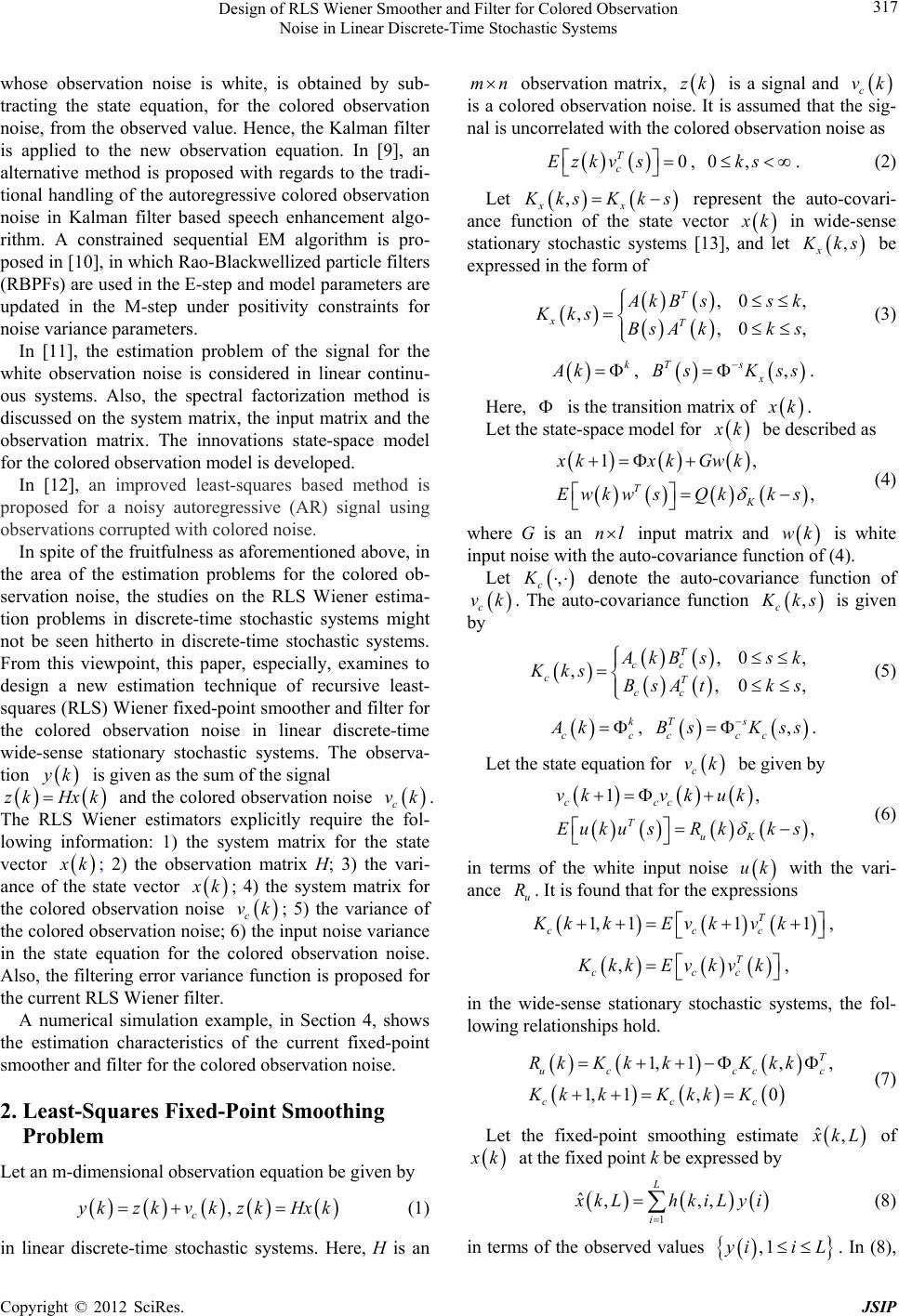 Design of RLS Wiener Smoother and Filter for Colored Observation Noise in Linear Discrete-Time Stochastic Systems 317 whose observation noise is white, is obtained by sub- tracting the state equation, for the colored observation noise, from the observed value. Hence, th e Kalman filter is applied to the new observation equation. In [9], an alternative method is proposed with regards to the tradi- tional handling of the autoregressive colored observation noise in Kalman filter based speech enhancement algo- rithm. A constrained sequential EM algorithm is pro- posed in [10], in which Rao-Blackwellized particle filters (RBPFs) are used in the E-step and model parameters are updated in the M-step under positivity constraints for noise variance parameters. In [11], the estimation problem of the signal for the white observation noise is considered in linear continu- ous systems. Also, the spectral factorization method is discussed on the system matrix, the input matrix and the observation matrix. The innovations state-space model for the colored observation model is developed. In [12], an improved least-squares based method is proposed for a noisy autoregressive (AR) signal using observations corrupted with colored noise. In spite of the fruitfulness as aforementioned above, in the area of the estimation problems for the colored ob- servation noise, the studies on the RLS Wiener estima- tion problems in discrete-time stochastic systems might not be seen hitherto in discrete-time stochastic systems. From this viewpoint, this paper, especially, examines to design a new estimation technique of recursive least- squares (RLS) Wiener fix ed-point smoother and filter for the colored observation noise in linear discrete-time wide-sense stationary stochastic systems. The observa- tion k Hx is given as the sum of the signal and the colored observation noise zk k c vk. The RLS Wiener estimators explicitly require the fol- lowing information: 1) the system matrix for the state vector k; 2) the observation matrix H; 3) the vari- ance of the state vector k; 4) the system matrix for the colored observation noise ; 5) the variance of the colored observation noise; 6) the input no ise variance in the state equation for the colored observation noise. Also, the filtering error variance fun ction is proposed for the current RLS Wiener filter. c vk A numerical simulation example, in Section 4, shows the estimation characteristics of the current fixed-point smoother and filter for the colored observation noise. 2. Least-Squares Fixed-Point Smoothing Problem Let an m-dimensional observation equation be given by , c kzkvkzkHxk (1) in linear discrete-time stochastic systems. Here, H is an mn observation matrix, is a signal and zk c vk is a colored observation noise. It is assumed that the sig- nal is uncorrelated with the colored observation noise as 0 T c Ezkv s , . (2) 0,ks Let , xx ksK k s represent the auto-covari- ance function of the state vector k in wide-sense stationary stochastic systems [13], and let , x ks be expressed in the form of ,0 , ,,0 , T xT kBss k Kks BsA kks (3) k Ak , , Ts x Bs Kss . Here, is the transition matrix of k. Let the state-space model for k be described as 1, , TK xkxk Gwk EwkwsQkk s (4) where G is an nl input matrix and is white input noise with the auto-covariance function of (4). wk Let , c K denote the auto-covariance function of c vk. The auto-covariance function , c ks is given by ,0 , ,,0 , T cc cT cc kBss k KksBsAtk s (5) k cc Ak , . , Ts ccc Bs Kss Let the state equation for be given by c vk 1, , ccc TuK vkvk uk EukusR kks (6) in terms of the white input noise with the vari- ance . It is found that for the expressions uk u R 1, 111 T ccc Kk kEvkvk , ,T ccc kkEvkvk , in the wide-sense stationary stochastic systems, the fol- lowing relationships hold. 1, 1,, 1, 1,0 T uc cc ccc Rk KkkKkk KkkKkk K c (7) Let the fixed-point smoothing estimate ˆ, kL of k at the fixed point k be expressed by 1 ˆ,,, L i kL hkiLyi (8) in terms of the observed values . In (8), ,1yii L Copyright © 2012 SciRes. JSIP 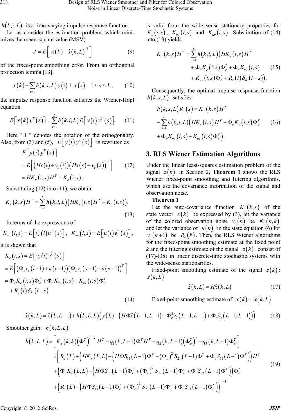 Design of RLS Wiener Smoother and Filter for Colored Observation Noise in Linear Discrete-Time Stochastic Systems Copyright © 2012 SciRes. JSIP 318 ,,hkiL is a time-varying impulse response function. is valid from the wide sense stationary properties for , c is , , vu is and , uv is . Substitution of (14) into (13) yields Let us consider the estimation problem, which mini- mizes the mean-square value (MSV) 2 ˆ,JE xkxkL (9) 1 ,,,, ,, ,. L TT xx i T ccc cvu T uvc uK KksH hkiLHKisH KisKis isR ii s (15) of the fixed-point smoothing error. From an orthogonal projection lemma [13], 1 ,, L i khkiLyiy s1, L , (10) Consequently, the optimal impulse response function ,,hksL satisfies the impulse response function satisfies the Wiener-Hopf equation Ex 1,, . L TT i ky shkiLEyiys , T c (11) 1 ,, , ,, ,, ,,. T ux LTT cc c i T cvuuv c hksLR sKksH hkiL HKisHKis KisKis (16) Here “” denotes the notation of the orthogonality. Also, from (3) and (5), is rewritten as T Eyiys ,,. T T cc T xc Eyiy s EHxivi Hxs vs HKi sHKi s (12) 3. RLS Wiener Estimation Algorithms Substituting (12) into (11), we obtain 1 ,,,, L T xx i . Under the linear least-squares estimation problem of the signal zk in Section 2, Theorem 1 shows the RLS Wiener fixed-point smoothing and filtering algorithms, which use the covariance information of the signal and observation noise. ks , vu HhkiL HK isHKis (13) Theorem 1 Let the auto-covariance function , x In terms of the expressions of T c E vius , ,T uv c isEuiv s , is it is shown that , cc Kis Ki Ri 11 11 ,,, T ccc T cc cc T c cvuuvc uK Evivs Eviuivs us sK isK is is T (14) ks of the state vector k be expressed by (3), let the variance of the colored observation noise c v be k , c kk and let the variance of uk in the state equation (6) for 1 c vk be k u R. Then, the RLS Wiener algorithms for the fixed-point smoothing estimate at the fixed point k and the filtering estimate of the signal consist of (17)-(38) in linear discrete-time stochastic systems with the wide-sense stationarities. zk Fixed-point smoothing estimate of the signal zk: ˆ,zkL ˆ ˆ,zkL HxkL , (17) Fixed-point smoothing estimate of k: ˆ, kL 223 ˆˆˆˆ ,,1 ,,1,11,11,1 cc xkLxkL hkLLyLHxLLvLLvLL ˆ TT T (18) Smoother gain: ,,hkLL 2 123 2 1121 31 2 1222 32 2 132333 ,,,, 1, 1, 1 ,1 11 ,1 11 111 Lk TT TTTT xcc TT uxc c TTT ccccc cc c TTT uccccc hkLLKkkH qkLH qkLqkL RLHKLLHSLSLS LH KLLHS LS LSL RLHS LSLSL 1 (19) 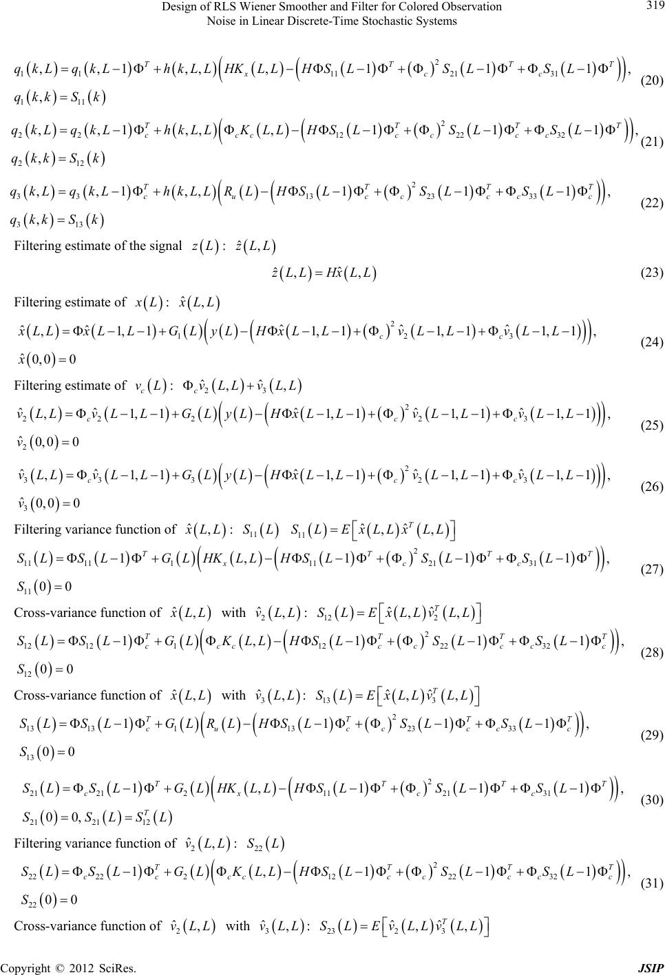 Design of RLS Wiener Smoother and Filter for Colored Observation Noise in Linear Discrete-Time Stochastic Systems 319 2 1 1112131 111 ,,1,,,111 , TTT xcc q kLq kLhkLLHKLLHSLSLSL qkkSk , T (20) 2 2 2122232 212 ,,1,, ,111 , TTT ccc cccc qkLqkLhkLLKLLHS LSLSL qkkS k , T (21) 2 3 3132333 313 ,,1,,11 1 , TTT cu cccc qkLqkLhkLLRLHS LSLS L qkkSk , T c (22) Filtering estimate of the signal : zL ˆ,zLL ˆ ˆ,zLL HxLL, (23) Filtering estimate of L: ˆ, LL 2 12 ˆˆˆˆˆ ,1,11,11,1 1,1 ˆ0,0 0 cc xLL xLLGLyLHxLLvLLvLL x 3 , (24) Filtering estimate of c vL: 23 ˆˆ ,, cvLL vLL 2 22 223 2 ˆˆ ˆˆˆ ,1,11,11,1 1,1 ˆ0,0 0 ccc vLLvLLGLyLHxLLvL LvL L v , (25) 2 33 323 3 ˆˆˆˆ ˆ ,1,11,11,1 1,1 ˆ0,0 0 ccc vLLvLLGLyLHxLLvLLvLL v , (26) Filtering variance function of ˆ, LL : 11 SL 11 ˆˆ ,,SL ExLLxLL T 11 11 1112131 11 1,11 00 TTT xcc SLSLGLHKLL HSLSLSL S 21, T (27) Cross-variance function of ˆ, LL with 2 ˆ,vLL : 12 2 ˆˆ ,, T SL ExLLvLL 12 12 1122232 12 1,11 00 TTT ccccc cc SLSLGLKLLHSLSLSL S 21, T c (28) Cross-variance function of ˆ, LL with 3 ˆ,vLL : 13 3 ˆˆ ,, T SL ExLLvLL 2 13 13 1132333 13 111 00 TTT cucc cc SLSLGLRL HSLSLSL S 1, T c (29) 2 21 212112131 2121 12 1,11 00, TTT cx cc T SLSLGLHKLLHSLSLSL SSLSL 1, T (30) Filtering variance function of : 2 ˆ,vLL 22 SL 2 22 222122232 22 1,11 00 TTT cccccccc SLSLGLKLL HSLSLSL S 1, T c (31) Cross-variance function of with 2 ˆ,vLL 3 ˆ,vLL : 232 3 ˆˆ ,, T SLEvLLvLL Copyright © 2012 SciRes. JSIP  Design of RLS Wiener Smoother and Filter for Colored Observation Noise in Linear Discrete-Time Stochastic Systems Copyright © 2012 SciRes. JSIP 320 2 23 232132333 23 111 00 TTT ccucc cc SLSLGLRL HSLSLSL S 1, T c (32) 2 31 313112131 3131 13 1,11 00, TTT cx cc T SLSLGLHKLL HSLSLSL SSLSL 1, T (33) 2 32 323122232 3232 23 1,11 00, TTT cccccc cc T SLSLGLKLL HSLSLSL SSLSL 1, T c (34) Filtering variance function of : 3 ˆ,vLL 3333 ˆˆ ,,SL EvLLvLL T 33 33 3132333 33 111 00 TTT ccucc cc SLSLGLRL HSLSLSL S 21, T c (35) Filter gain for ˆ, LL : 1 GL 2 1111213 2 1121 31 2 1222 32 1 2 1323 33 ,11 1 ,1 11 ,1 11 111 TTTTT xc TT uxc c TTT cccccccc TTT uccccc GLKLLH SLHSLSL RLHKLLHS LSLSLH KLLHS LSLSL RLHS LSLSL c TT T TT T (36) Filter gain for : 2 ˆ,vLL 2 GL 2 2212223 2 1121 31 2 1222 32 1 2 132333 ,11 1 ,1 11 ,1 11 111 TTTTT cccccc c TT uxc c TTT cccccccc TTT uccccc GLKLLS LHS LSL RLHKLLHS LSLSLH KLLHS LSLS L RLHS LSLSL (37) Filter gain for 3 ˆ,vLL : 3 GL 2 3313233 2 1121 31 2 1222 32 1 2 1323 33 111 ,1 11 ,1 11 111 TT TT ucccc c TT uxc c TTT ccccccc c TTT uccccc GLRLS LHSLS L RLHKLLHSLSLSLH KLLHS LSLS L RLHS LSLSL TT T (38) Proof of Theorem 1 is deferred to the Appendix. Figure 1 illustrates the flowchart for the filtering and fixed-point smoothing algorithms of Theorem 1. The calculating steps are divided into two parts corresponding to the filter and the fixed-point smoother. From Theorem 1, it is found that the filtering error variance function z PL of the signal is given by zL 11 ,1 TT zz PLK LLHSLH , (39) where , z LL represents the variance function of zL. 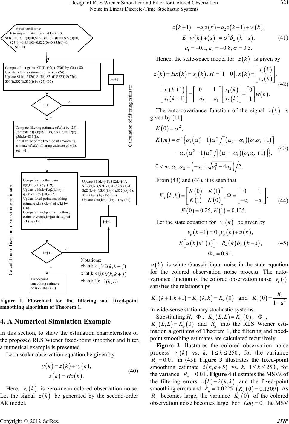 Design of RLS Wiener Smoother and Filter for Colored Observation Noise in Linear Discrete-Time Stochastic Systems 321 otations: zhat ( k , k+ j): ),( ˆjkkz xhat(k,k+j ): ),( ˆjkkx zhat(k,L): ),( ˆLkz Compute filter gains G1(i), G2(i), G3(i) by (36)-(38). Update filtering estimates of x(j) by (24). Update S11(i),S12(i),S13(i),S21 (i), S22(i),S(23 (i), S31(i),S32(i),S33(i) by (27)-(35). Compute smoother gain h(k,k+j,k+j) by (19). Update q1(k,k+j),q2(k,k+j), q3(k,k+j) by (20)-(22). Update fixed-point smoothing estimate xhat(k,k+j) of x( k) b y (18). Compute fixed-point smoothing estimate zhat (k,k+j)of th e signal z(k) by (17). Initial conditions: filtering estimate of x(k) at k=0 is 0, S1 1(0)=0, S12(0)=0,S13(0)=0,S21(0)=0,S22(0)=0, S23(0)=0,S31(0)=0,S32(0)=0,S33(0)=0. Set i=1. i:k< = i=i+1 Compute f iltering estimate of z( k) by ( 23) . Compute q1(k,k)=S11(k), q2(k,k)=S12(k), q3(k,k)=S13(k). Initial value of the fixed-point smoothing estimate of x(k): filtering estimate of x(k). Set j=1. k+j:L Fixed-point smoothing estimate o f z(k ): zhat(k,L) < = j=j+1 Update S11(k+j-1),S12(k+j-1), S13(k+j-1),S21(k+j-1),S22(k+j-1), S(23(k+j-1),S31(k+j-1),S32(k+j-1), S33(k+j-1 ) by (27)-(35). Update xhat(k+j-1,k+j-1) by (24). Calculation of fixed-point smoothing estimate Calcu la t i o n of filter in g est im a te Figure 1. Flowchart for the filtering and fixed-point smoothing algorithm of Theorem 1. 4. A Numerical Simulation Example In this section, to show the estimation characteristics of the proposed RLS Wiener fixed-point smoother and filter, a numerical example is presented. Let a scalar observation equation be given b y , . c ykzkvk zk Hxk (40) Here, is zero-mean colored observation noise. Let the signal be generated by the second-order AR model. c vk zk 12 2 12 11 , 0.1,0.8, 0.5. K zkazk azkwk Ewkwsk s aa , (41) Hence, the state-space model for zk is given by 1 12 11 2221 ,10, 101 0. 11 , k zkHxkxkHxk k xkxk wk xk xk aa (42) The auto-covariance function of the signal zk is given by [ 1 1 ] 2 22 1212 1 21 2 21221 12 2 1211 2 0, 11 11 0,,4 2. m m K Km maaa , (43) From (43) and (44), it is seen that 21 01 01 ,, 10 00.25,1 0.125. x KK Kkk , Ka KK a (44) Let the state equation for c vk be given by 1, , 0.91. ccc TuK c vkvkuk EukusR kks (45) uk is white Gaussin input noise in the state equation for the colored observation noise process. The auto- variance fun ction of the colored observation no ise c v satisfies the relationships 1, 1,0 cc KkkKkk K c and 2 01u cR Ka in wide-sense stationary stochastic systems. Substituting H, , , xx KLL K 0, c, ,0 c KLL Kc and u into the RLS Wiener esti- mation algorithms of Theorem 1, the filtering and fixed- point smoothing estimates are calculated recursively. R Figure 2 illustrates the colored observation noise process c vk vs. k, 125k0 , for the variance 0.01 u R in (45). Figure 3 illustrates the fixed-point smoothing estimate ,5 k ˆ zk 01 vs. k, , for the variance u 125k 0 0.R . Figure 4 illustrates the MSVs of the filtering errors ˆ,zkk0.0225 zk R and the fixed-point smoothing errors and u . As u becomes large, the variance of the colored observation noise becomes large. For , the MSV 00.1309 0Lag c K 0Rc K Copyright © 2012 SciRes. JSIP 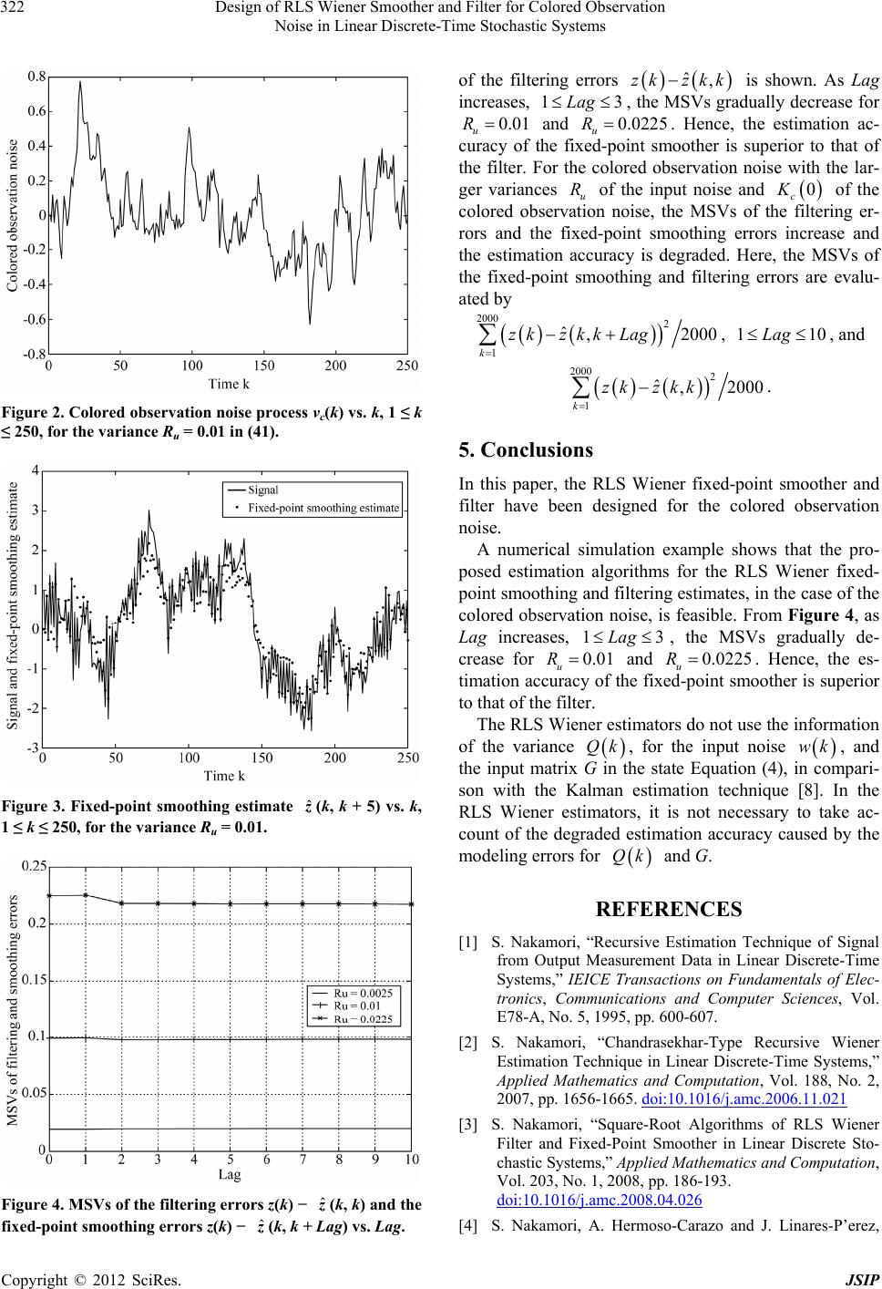 Design of RLS Wiener Smoother and Filter for Colored Observation Noise in Linear Discrete-Time Stochastic Systems 322 Figure 2. Colored observation noise process vc(k) vs. k, 1 ≤ k ≤ 250, for the variance Ru = 0.01 in (41). Figure 3. Fixed-point smoothing estimate (k, k + 5) vs. k, 1 ≤ k ≤ 250, for the variance Ru = 0.01. ˆ z Figure 4. MSVs of the filtering errors z(k) − (k, k) and the fixed-point smoothing errors z(k) − (k, k + Lag) vs. Lag. ˆ z ˆ z of the filtering errors ˆ,zk zkk 3 is shown. As Lag increases, 1Lag , the MSVs gradually decrease for 0.01 u R and u0.0225R . Hence, the estimation ac- curacy of the fixed-point smoother is superior to that of the filter. For the colored observation noise with the lar- ger variances u of the input noise and R 0 c K of the colored observation noise, the MSVs of the filtering er- rors and the fixed-point smoothing errors increase and the estimation accuracy is degraded. Here, the MSVs of the fixed-point smoothing and filtering errors are evalu- ated by 2000 2 1 ˆ, 2000 k zkzkk Lag , , and 11Lag0 2000 2 1 ˆ,2000 k zk zkk 3 . 5. Conclusions In this paper, the RLS Wiener fixed-point smoother and filter have been designed for the colored observation noise. A numerical simulation example shows that the pro- posed estimation algorithms for the RLS Wiener fixed- point smoothing and filtering estimates, in the case of the colored observation noise, is feasible. From Figure 4, as Lag increases, 1Lag 0.01 , the MSVs gradually de- crease for u R and . Hence, the es- timation accuracy of the fixed-point smoother is superior to that of the filter. 0.0225 uR The RLS Wiener estimators do not use the information of the variance Qk, for the input noise wk , and the input matrix G in the state Equation (4), in compari- son with the Kalman estimation technique [8]. In the RLS Wiener estimators, it is not necessary to take ac- count of the degraded estimation accuracy caused by the modeling errors for Qk and G. REFERENCES [1] S. Nakamori, “Recursive Estimation Technique of Signal from Output Measurement Data in Linear Discrete-Time Systems,” IEICE Transactions on Fundamentals of Elec- tronics, Communications and Computer Sciences, Vol. E78-A, No. 5, 1995, pp. 600-607. [2] S. Nakamori, “Chandrasekhar-Type Recursive Wiener Estimation Technique in Linear Discrete-Time Systems,” Applied Mathematics and Computation, Vol. 188, No. 2, 2007, pp. 1656-1665. doi:10.1016/j.amc.2006.11.021 [3] S. Nakamori, “Square-Root Algorithms of RLS Wiener Filter and Fixed-Point Smoother in Linear Discrete Sto- chastic Systems,” Applied Mathematics and Computation, Vol. 203, No. 1, 2008, pp. 186-193. doi:10.1016/j.amc.2008.04.026 [4] S. Nakamori, A. Hermoso-Carazo and J. Linares-P’erez, Copyright © 2012 SciRes. JSIP 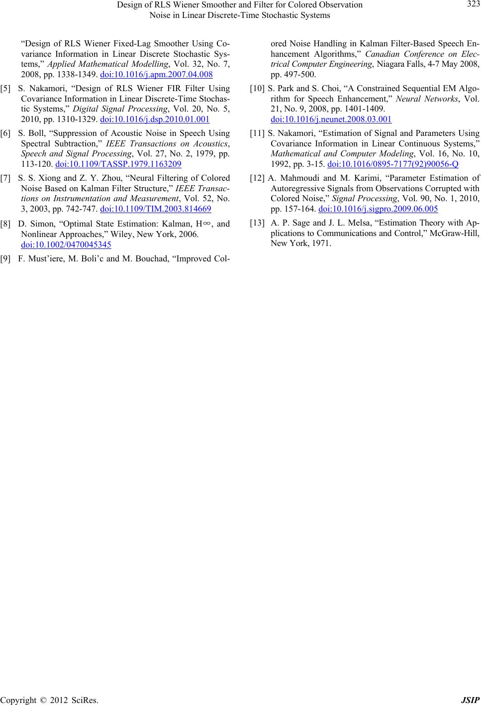 Design of RLS Wiener Smoother and Filter for Colored Observation Noise in Linear Discrete-Time Stochastic Systems Copyright © 2012 SciRes. JSIP 323 “Design of RLS Wiener Fixed-Lag Smoother Using Co- variance Information in Linear Discrete Stochastic Sys- tems,” Applied Mathematical Modelling, Vol. 32, No. 7, 2008, pp. 1338-1349. doi:10.1016/j.apm.2007.04.008 [5] S. Nakamori, “Design of RLS Wiener FIR Filter Using Covariance Information in Linear Discrete-Time Stochas- tic Systems,” Digital Signal Processing, Vol. 20, No. 5, 2010, pp. 1310-1329. doi:10.1016/j.dsp.2010.01.001 [6] S. Boll, “Suppression of Acoustic Noise in Speech Using Spectral Subtraction,” IEEE Transactions on Acoustics, Speech and Signal Processing, Vol. 27, No. 2, 1979, pp. 113-120. doi:10.1109/TASSP.1979.1163209 [7] S. S. Xiong and Z. Y. Zhou, “Neural Filtering of Colored Noise Based on Kalman Filter Structure,” IEEE Transac- tions on Instrumentation and Measurement, Vol. 52, No. 3, 2003, pp. 742-747. doi:10.1109/TIM.2003.814669 [8] D. Simon, “Optimal State Estimation: Kalman, H∞, and Nonlinear Approaches,” Wiley, New York, 2006. doi:10.1002/0470045345 [9] F. Must’iere, M. Boli’c and M. Bouchad, “Improved Col- ored Noise Handling in Kalman Filter-Based Speech En- hancement Algorithms,” Canadian Conference on Elec- trical Computer Engineering, Niagara Falls, 4-7 May 2008, pp. 497-500. [10] S. Park and S. Choi, “A Constrained Sequential EM Algo- rithm for Speech Enhancement,” Neural Networks, Vol. 21, No. 9, 2008, pp. 1401-1409. doi:10.1016/j.neunet.2008.03.001 [11] S. Nakamori, “Estimation of Signal and Parameters Using Covariance Information in Linear Continuous Systems,” Mathematical and Computer Modeling, Vol. 16, No. 10, 1992, pp. 3-15. doi:10.1016/0895-7177(92)90056-Q [12] A. Mahmoudi and M. Karimi, “Parameter Estimation of Autoregressive Signals from Observations Corrupted with Colored Noise,” Signal Processing, Vol. 90, No. 1, 2010, pp. 157-164. doi:10.1016/j.sigpro.2009.06.005 [13] A. P. Sage and J. L. Melsa, “Estimation Theory with Ap- plications to Communications and Control,” McGraw-Hill, New York, 1971.  Design of RLS Wiener Smoother and Filter for Colored Observation Noise in Linear Discrete-Time Stochastic Systems 324 Appendix Proof of Theorem 1 If we subtract the equation obtained by putting in (16) from (16), we h ave 1LL 1 1 ,,,,1, ,,,, ,,,, 1,,,,, TT uxccvc LTT xccccvu uvc i hksLhksLR shkLLHKLsHKLsKLs hkiLhkiLHKisHK isKisKis vu T .0 (A-1) for ,0 uv KLs From (6) and , it is shown that , vu Kss , vu Ls satisfies 11 ,, LsLs Ls vucvucucu LsKssR sR s . (A-2) Let us introduce the following auxiliary functions 1,1JsL , 2,1JsL and 3,1JsL as follows. 1 11 1 ,1,,1 ,,,, L sTT T uxx ccccvuuv i JsLRsKssHJiLHKisHKisKisKis , T c , T . T c (A-3) 1 22 1 ,1,,1 ,,,, L sTT T ucc cxccccvuuvc i JsLRsKssJiLHKisHKisKisKis (A-4) 1 33 1 ,1,1 ,,,, L sTT ucuxccccvu uv i JsLR sR sJ iLHKisHK isKisKis (A-5) From (A-1), (A-3), (A-4) and (A-5), we obtain 1 123 ,,,, 1,,, 1,1,1. LL L cc hksLhksLhkLL HJ sLJsLJsL (A-6) If we subtract 1,1 u sLRs from 1,u sLRs , we have 11 1 1 11 1 ,,1,,,, , ,,1 ,,,,. TT uxccccvuuv LTT T xccccvuuvc i JsLJsLRsJLLHKLsHKLsK LsK Ls J iLJiLHKisHKisKisKis T c (A-7) From (A-3)-(A-5) and (A-7), we obtain 1 11 1123 ,,1,,1,1,1 LL L cc JsLJsLJLLH JsLJsLJsL . (A-8) If we subtract 2,1 sL Rs from 2, sLR s , we ha ve 22 2 1 22 1 ,,1,,,, , ,,1,,, ,. TT uxccccvuuv LTT T xccccvuuvc i JsL JsLRsJLLHKLsHKLsK Ls K Ls J iLJ iLHK isHKisKisKis T c (A-9) From (A-3)-(A-5) and (A-9), we obtain 1 22 2123 ,,1,,1,1,1 LL L cc J sLJ sLJ LLHJsLJ sLJsL . (A-10) If we subtract 3,1 u sLR s from 3,u sLRs , we ha ve 33 3 1 33 1 ,,1,,,, , ,,1,,, ,. TT uxccccvuuv LTT T xccccvu uvc i JsLJsLRsJLLHKLsHKLsKLsK Ls J iLJ iLHKisHK isKisKis T c (A-11) From (A-3)-(A-5) and (A-11), we obtain 1 33 3123 ,,1 ,,1,1,1 LL L cc J sLJ sLJ LLHJsLJsLJ sL . (A-12) By putting 1 L in (A-3), we have Copyright © 2012 SciRes. JSIP  Design of RLS Wiener Smoother and Filter for Colored Observation Noise in Linear Discrete-Time Stochastic Systems 325 1 1 (1) 1 1 12 (1) 1 1 1, 11 1, 1,1, 1, 1, 1,1 1, 1,111. u L TTT T xccccvu uvc i LL LT TTTTTT xcccc uvcc i JL LRL KLLHJiL HKiLHKiLKiLKiL KLLHJiL BiALHBiALBi (A-13) Here, from (6), the relationships ,10 vu KiL,11iL , and , are taken into accounts. 2 ,1 L T uvuv c KiL Bi i T uvu v Bi Ri By introducing the functions 1 11 1 1 1,1 L i rLJiL HBi . , (A-14) 1 12 1 1 1,1 L ccv i rLJiL Bi , (A-15) 1 13 1 1 1,1 L uv i rLJiL Bi , (A-16) (A-13) can be written as 1 1 1 1112 12 1, 111, 1 1111 1 LT ux L TT TTT cc c JLL RLKLL H rL ALHrL ALrL (A-17) By putting 1 L in (A-4), we have 1 2 1 2 1 1, 111,1 ,1,1,1,1 ,1 LT ucc c LTT xccccvu uvc i JL LRLKLL JiLHKiLHKiLK iLKiL . T . (A-18) By introducing the functions 1 21 2 1 1,1 L i rLJiL HBi , (A-19) 1 22 2 1 1,1 L cc i rLJiL Bi , (A-20) 1 23 2 1 1,1 L uv i rLJiL Bi , (A-21) (A-18) can be written as 1 2 1 2122 23 1, 111, 1 1111 1 LT ucc c L TT TTT ccc JL LRLKL L rL ALHrL ALrL (A-22) By putting 1 L in (A-5), we have 1 3 1 3 1 1, 111 ,1,1,1,1 ,1 LT ucu LTT xccccvuuv i JLLRL RLH JiLHKiLHKiLK iLK iL . T c (A-23) By introducing the functions Copyright © 2012 SciRes. JSIP  Design of RLS Wiener Smoother and Filter for Colored Observation Noise in Linear Discrete-Time Stochastic Systems 326 1 31 3 1 1,1 L i rLJiLHBi . , (A-24) 1 32 3 1 1,1 L cc i rLJiL Bi , (A-25) 1 33 3 1 1,1 L uv i rLJiLBi , (A-26) (A-23) can be written as 1 3 1 313233 1, 111 1111 1 L cu L TT TTT cc c JL LRLRL rLALH rLALrL (A-27) If we subtract from and use (A-8), (A-14), (A -19) and (A-24), we ob tain 11 2rL 11 1rL 2 11 11111 1 21(1) 11123 1 11 1112131 121,11 ,1,2 1,111,1, 2, 2, 2 1,11222 . L i LLLL cc i LL L cc rLrLJLLHBLJiLJiLHBi LLHBLJLLHJiLJiLJiL HBi JLLHBLHrLr Lr L (A-28) If we subtract from and use (A-8), (A-15), (A -20) and (A-25), we ob tain 12 2rL 32 33 12 1rL 2 12 12111 1 11 11222 121,1 1,1,2 1,11222 . L cc cc i LL L ccc c rLrLJLLBLJiLJiLBi JLLBLHr LrLrL (A-29) If we subtract from and use (A-8), (A-16), (A -21) and (A-26), we ob tain 13 2rL 13 1rL 2 13 13111 1 11 11323 121,11 ,1,2 1,11222 . L uv uv i LL L uvc c rLrLJL LBLJiLJiLBi JLLBLHrLr Lr L (A-30) If we subtract 21 2rL from 21 1rL and use (A -10), (A-14), (A-19) and (A-24), we obtain 2 21 21222 1 11 21121 121,11 ,1,2 1,11222 . L i LL L cc rLrLJL LHBLJiLJiLHBi JL LHBLHrLrLrL 31 32 33 (A-31) If we subtract from and use (A-10), (A-15), (A-20) and (A-25), we obtain 22 2rL 22 1rL 2 22 22222 1 11 21222 121,11,1,2 1,11222. L cc cc i LL L ccc c rLrLJLLBLJiLJiLBi JL LBLHrLrLrL (A-32) If we subtract from and use (A-10), (A-16), (A-21) and (A- 26), we obtain 23 2rL 23 1rL 2 23 23222 1 11 21323 121,11 ,1,2 1,11222 . L uv uv i LL L uvc c rLrLJL LBLJiLJiLBi JL LBLHrLrLrL (A-33) If we subtract 31 2rL from 31 1rL and use (A-12), (A -14), (A-19) and (A-24), we obtain Copyright © 2012 SciRes. JSIP  Design of RLS Wiener Smoother and Filter for Colored Observation Noise in Linear Discrete-Time Stochastic Systems Copyright © 2012 SciRes. JSIP 327 31 32 2 31 31333 1 11 31121 121,11 ,1,2 1,11222 . L i LL L cc rLrLJL LHBLJiLJiLHBi JL LHBLHrLrLrL (A-34) If we subtract from and use (A-12), (A-15), (A-20) and (A- 25), we obtain 32 2rL 32 1rL 2 32 32333 1 11 31222 121,1 1,1,2 1,11222. L cc cc i LL L ccc c rLrLJLLBLJiLJiLBi JLLBLHrLr Lr L (A-35) If we subtract 33 2rL from 33 1rL and use (A-12), (A-16), (A-21) and (A-26), we obtain 2 33 33333 1 11 31323 121,11 ,1,2 1,11222 . L uv uv i LL L uvc c rLrLJL LBLJiLJiLBi JLLB LHrLr LrL 33 (A-36) Here, the initial values of , , 11 rk 12 rk 13 rk, 21 rk , 22 rk, 23 rk, 31 rk, and , at 32 rk 33 rk 0k are , , , 21 11 00r 12 00r 13 r00r 00 , 22 r00 , 00 23 r , 31 00r , and 0 32 r0 00 33 r from (A-14)-(A-16), (A-19)-(A-21) and (A-24)-(A-26). Let us introduce the functions 11 1112 121313 21 21222223 23 31 31323233 33 ,, ,, ,, LL LT LT LT cc , . L LL LT LT LT ccccc LL LT LT LT cccc SL rLSL rLSLrL SL rLSL rLSL rL SL rLSL rLSL rL c (A-37) Substituting (A-28)-(A-36) into (A-37) and introducing 11 ,, L GL JLL 22 , L c GL JLL and 3 GL 3, L c LL, we obtain the recursive Equations (27)-(35) for 11 SL, 12 SL, 13 SL 21 SL 22 S, , , L 23 SL, , and . 31 SL 32 S L 33 SL From (A-17), (A-22) and (A-27), , 1 GL 2 GL and GL 3 are formulated as 1 1111213 1 1112 13 , ,, TLTTLT TLT xcc TTT xcu GLKLLHr LA LHrLA LrLALRL KLLHSLHS LSLRL cu (A-38) 1 2212223 1 2122 23 , ,, TLTTLT TLT ccccccccu TTT ccc u GLKLLrLALHrLALrLALRL KLLS LHS LSLRL (A-39) 1 3313233 1 313233. LTTLTTL T uc cccccu TT ucu GLRLrLALHrLA LrLALRL RLSLHSLSLRL (A-40) Substituting (27)-(29) into (A-38), after some manipu- lations, we obtain (36). Similarly, from (30)-(32) and (A-39), (37) is obtained. Also, by substituting (33)-(35) into (A-40), (38) is obtained. 21 ,,,, Li T cc c i PkLhkiLKii , (A-42) 31 ,,, Li T uc i PkLhkiLRi , (A-43) Putting 11 ,,,, Li T x i PkLhkiLHKii , (A-41) rom (3), (5) and (16), ,,hkLL satisfies f  Design of RLS Wiener Smoother and Filter for Colored Observation Noise in Linear Discrete-Time Stochastic Systems 328 1 1 1 123 ,, ,, ,,,, (,) ,,,,. LLi TTTTTT T ucccc uc i L kiLiL TTTTTTTTT xxccccc i LkLL L TTTTTT xcc hkLLRL BkALHhkiLHBiALHBiALRi KkkHhkiLHKiiHK iiRi KkkHPkLH PkLPkL Li uc (A-44) Subtracting from and using (A-6), (A-14), (A-19) and (A-24), we obtain 1,1PkL 1,PkL 1 11 1 11 123 1 1 1121 31 ,, 1,,,,,,, 1, ,,,,,,1, 1,1, ,,,111 . L Li TT xx i L i TLLL xccx i L TL LL xcc PkLPkLhkLLHKLLhkiLhkiLHK ii hkLLHKLLhkLLHJ iLJiLJiLHKii hkLLHKLLHrLrLrL T (A-45) Subtracting from and u sing (A-6), (A-15), (A- 20) and (A-25), we obtain 2,1PkL 2,PkL 1 22 1 1 1222 32 ,,1,,,,,,, 1, ,,,111. L i TT ccccc c i L TL LL cc ccc P kLP kLhkLLKLLhkiLhkiLKii hkLLK LLHrLrLrL (A-46) Subtracting 3,1PkL from 3,PkLand using (A-6), (A-16), (A-21) and (A-26), we obtain 1 33 1 1 1323 33 ,,1,, ,,,,1 ,,111. L i TT uc uc i L TL LL ucc c P kLP kLhkLLRLhkiLhkiLRi hkLL R LHrLrLrL (A-47) Putting 11 ,, T qkL PkL, (A-48) and using (A-37), we obtain (2 0). Putting 22 ,, T c qkL PkL, (A-49) and using (A-37), we obtain (2 1). Putting 33 ,, T c qkL PkL , (A-50) and using (A-37), we obtain (2 2). From (16) and (A -3), we obtain 1 ,, , k hkskJ sk . (A-51) From (A-14), (A-37), (A-41) and (A-48), 1,qkk is derived as 11 1 1 12 11 ,, ,, . k T ki kT x i k kT c qkk Pkk JikHKii rk Sk From (A-15), (A-37), (A-42) and (A-49), 2,qkk is derived as 22 1 1 12 12 ,, ,, . k T c ki kT ccc c i k kT c qkkPkk JikKii rk Sk k T (A-53) Similarly, from (A-16), (A-37), (A-43) and (A-50), 3,qkk is derived as 33 1 1 13 12 ,, , . k T c ki kT ucc i k kT c qkk Pkk JikRi rk Sk k T ,. (A-54) From (A-44), (A-4 8), (A-49) and (A-50), we obtain k T (A-52) 123 ,, , ,, Lk TT ux TT c hkLLR LK kkH qkLH qkLqkL (A55) Substituting (20), (21) and (22) into (A-55), we obtain Copyright © 2012 SciRes. JSIP  Design of RLS Wiener Smoother and Filter for Colored Observation Noise in Linear Discrete-Time Stochastic Systems 329 (19) for the smoother gain . ,,hkLL From (8) and (A-51), the filtering estimate ˆ, LL of L becomes 1 11 ˆ,,,, LL L ii LLhLiL yiJiL yi . (A-56) Introducing 11 1, L i OL JiLyi , (A-57) we have 1 ˆ,L LLO L . (A-58) Subtracting 11OL from and using (A-8), we have 1 OL 1 1111 1 1 11 111 23 1 2 123 1,, ,1 ,,,1,1,1 ˆˆˆ ,1,111. L i LLL L cc i cc OL OLJLLyLJiLJiLyi LL yLJLLHJiLJiLJiLyi JLLyLHxL LvLvL (A-59) Here, the functions , , 2 ˆ,vLL 3 ˆ,vLL 2 OL L and are introduced as follows. 3 OL 223 ˆˆ ,,, V vLLOLvLL OL L 3c L (A-60) 22 1 33 1 ,, ,. i L i OL JiLyi OL JiLyi (A-61) From (A-58) and (A-59) with 11 , L GL JLL , we obtain (24) updating the filtering estimate ˆ, LL from ˆ1, 1xLL . The initial condition of (24) for ˆ, LL at L = 0 is 0,0 0 ˆ x from (A-57) and (A-58). Subtracting 1 2 OL from and using (A-10), (A-57), (A-58), (A-60) and (A-61), we have 2 OL 2222 2 1 1 2123 2 22 1,, ,1 ,111 ˆˆˆ ,1,11,1 L i LL L cc cc OL OLJLLyLJiLJiLyi JLLyLH OLOLOL JLLyLHxLLvL LvL L 3 1,1. 3 1,1. (A-62) Subtracting from and using (A-12), (A-57), (A-58), (A-60) and (A-61), we have 31OL 3 OL 3333 3 1 1 3123 2 32 1,, ,1 ,111 ˆˆˆ ,1,11,1 L i LL L cc cc OL OLJLLyLJiLJiLyi JLLyLH OLOLOL JLLyLHxL LvL LvL L (A-63) From (A-60) and (A-62) with 22 , L c GL JLL 2 ˆ,vLL 33 , L c GL JLL , we obtain (25) for the filtering estimate . Also, from (A-60) and (A-63) with , we obtain (26) for the filtering estimate . 3 ˆ,vLL ˆ, From (8), (A-6), (A-57), (A-58), (A-60) and (A-61), the fixed-point smoothing estimate kL is updated as 1 1 2 23 1 123 2 23 ˆˆ ,,1,,,,,,1 ˆˆˆ ,,1, 11, 11, 1 ,,,,11 1 ˆˆ ˆ ,,1, 11, 11, 1. L i cc LL L cc cc xkL xkLhkLLyLhkiLhkiLyi hkLLyLHxLLvLL vLL hkLLyLhkLLHOLOLOL hkLLyLHxLLvLL vLL (A-64) (Q.E.D.) Copyright © 2012 SciRes. JSIP
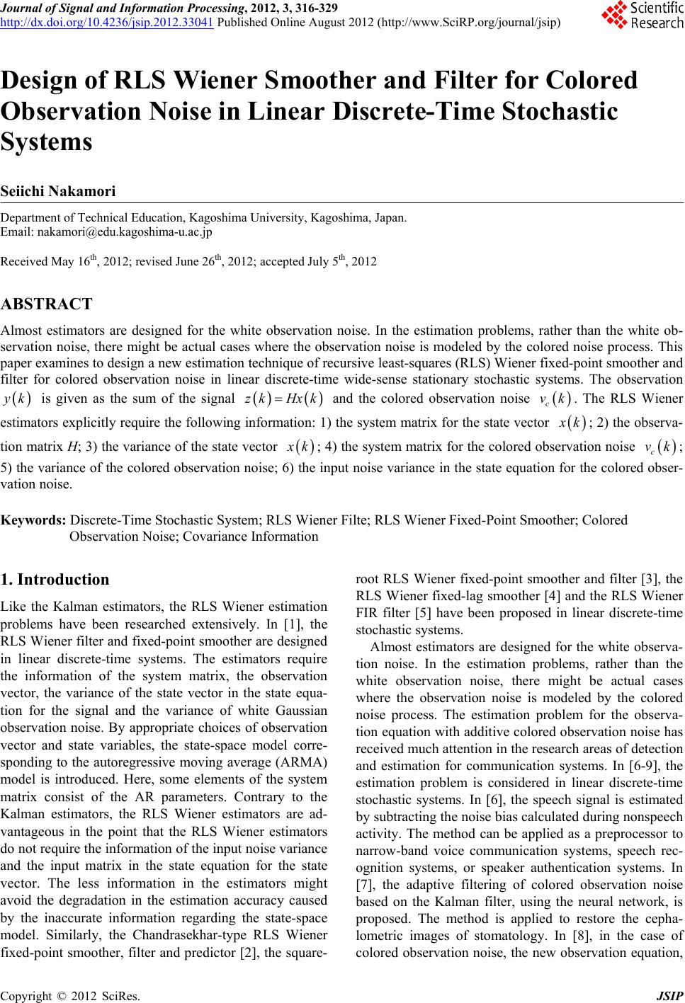
|