Applied Mathematics, 2010, 1, 128-136
doi:10.4236/am.2010.12017 Published Online July 2010 (http://www. SciRP.org/journal/am)
Vibration of Visco-Elastic Parallelogram Plate with
Parabolic Thickness Variation
Arun Kumar Gupta*, Anuj Kumar, Yogesh Kumar Gupta
Maharaj Singh College, Saharanpur, India
Received April 7, 2010; revised May 10, 2010; accepted May 17, 2010
Abstract
The main objective of the present investigation is to study the vibration of visco-elastic parallelogram plate
whose thickness varies parabolically. It is assumed that the plate is clamped on all the four edges and that the
thickness varies parabolically in one direction i.e. along length of the plate. Rayleigh-Ritz technique has been
used to determine the frequency equation. A two terms deflection function has been used as a solution. For
visco-elastic, the basic elastic and viscous elements are combined. We have taken Kelvin model for
visco-elasticity that is the combination of the elastic and viscous elements in parallel. Here the elastic ele-
ment means the spring and the viscous element means the dashpot. The assumption of small deflection and
linear visco-elastic properties of “Kelvin” type are taken. We have calculated time period and deflection at
various points for different values of skew angles, aspect ratio and taper constant, for the first two modes of
vibration. Results are supported by tables. Alloy “Duralumin” is considered for all the material constants
used in numerical calculations.
Keywords: Vibration, Parallelogram Plate, Visco-Elastic Mechanics, Parabolic Thickness, Aspect Ratio
1. Introduction
The materials are being developed, depending upon the
requirement and durability, so that these can be used to
give better strength, flexibility, weight effectiveness and
efficiency. So some new materials and alloys are utilized
in making structural parts of equipment used in modern
technological industries like space craft, jet engine, earth
quake resistance structures, telephone industry etc. Ap-
plications of such materials are due to reduction of
weight and size, low expenses and enhancement in effec-
tiveness and strength. It is well known that first few fre-
quencies of structure should be known before finalizing
the design of a structure. The study of vibration of skew
plate structures is important in a wide variety of applica-
tions in engineering design. Parallelogram elastic plates
are widely employed nowadays in civil, aeronautical and
marine structures designs. Complex shapes with variety
of thickness variation are sometimes incorporated to re-
duce costly material, lighten the loads, and provide ven-
tilation and to alter the resonant frequencies of the struc-
tures. Dynamic behavior of these structures is strongly
dependent on boundary conditions, geometric shapes,
material properties etc.
Dhotarad and Ganesan [1] have considered vibration
analysis of a rectangular plate subjected to a thermal
gradient. Amabili and Garziera [2] have studied trans-
verse vibrations of circular, annular plates with several
combinations of boundary conditions. Ceribasi and Altay
[3] introduced the free vibration analysis of super ellip-
tical plates with constant and variable thickness by Ritz
method. Gupta, Ansari and Sharma [4] have analyzed
vibration analysis of non-homogenous circular plate of
non linear thickness variation by differential quadrature
method. Jain and Soni [5] discussed free vibrations of
rectangular plates of parabolically varying thickness.
Singh and Saxena [6] discussed the transverse vibration
of rectangular plate with bi-directional thickness. Free
vibrations of non-homogeneous circular plate of variable
thickness resting on elastic foundation are discussed by
Tomar, Gupta and Kumar [7]. Yang [8] has considered
the vibration of a circular plate with varying thickness.
Gupta, Ansari and Sharma [9] discussed the vibration of
non-homogeneous circular Mindlin plates with variable
thickness. Bambill, Rossit, Laura and Rossi [10] have
analyzed transverse vibration of an orthotropic rectangu-
lar plate of linearly varying thickness with a free edge.
Sufficient work [11,12] is available on the vibration of
a rectangular plate of variable thickness in one direction,

A. K. GUPTA ET AL.
129
but none of them done on parallelogram plate. Recently
Gupta, Kumar and Gupta [13] studied the vibration of
visco-elastic parallelogram plate of linearly varying thic-
kness. A simple model presented here is to study the eff-
ect of parabolic thickness variation on vibration of visco-
elastic parallelogram plate having clamped boundary co-
nditions on all the four edges. The hypothesis of small
deflection and linear visco-elastic properties are made.
Using the separation of variables method, the governing
differential equation has been solved for vibration of vis-
co-elastic parallelogram plate. An approximate but quite
convenient frequency equation is derived by using Ray-
leigh-Ritz technique with a two-term deflection function.
It is assumed that the visco-elastic properties of the plate
are of the “Kelvin Type”. Time period and deflection fu-
nction at different point for the first two modes of vibra-
tion are calculated for various values of taper constant,
aspect ratio and skew angle and results are presented in
tabular form.
2. Equation of Transverse Motion
The parallelogram (skew) plate is assumed to be non-
uniform, thin and isotropic and the plate R be defined by
the three number a, b and θ as shown in Figure 1.
The skew coordinates are related to rectangular coor-
dinates are




sec,tan yyx 
The boundaries of the plate in skew coordinates are
ba 






,0,,0
The governing differential equation of transverse mo-
tion of visco-elastic parallelogram plate of variable thi-
ckness, ξ- and η- coordinates is given by [13]:
22
1cos
2
max
Tp hWdd

  (1)


Figure 1. Geometry of parallelogram plate.
and
22
22
1cos() 2(1)
2
sec(,,,)
VDW
WW Wdd
 











or
22
,,,
3
222
,,
22
,,,,
14sin 2(sin
2cos
cos)2(1sincos)
4sin
VDWWW
vWWv
WWWWdd
 
 
 









 




(2)
and
2Ď0
,t t
TpT

 (3)
A comma followed by a suffix denotes partial differ-
ential with respect to that variable. Here p2 is a constant.
Here solution w(ξ, η, t) can be taken in the form of
products of two functions as for free transverse vibration
of the parallelogram plate so that
)(),(),,(tTWtw





(4)
where T(t) is the time function and W is the maximum
displacement with respect to time t.
Assuming thickness variation of parallelogram plate
parabolically in ξ-direction as
})/(1{ 2
0ahh




(5)
where β is the taper constant in ξ-direction and

0
h
0 
h.
The flexural rigidity D of the plate can now be written
as
)1(12))/(1( 2323
0vaEhD 




, (6)
3. Solution and Frequency Equation
In using the Rayleigh-Ritz technique, one requires max-
imum strain energy be equal to the maximum kinetic
energy. So it is necessary for the problem consider here
that
0)( max 

TV

(7)
for arbitrary variations of W satisfying relevant geomet-
rical boundary conditions.
For a parallelogram plate, clamped (c) along all the
four edges, the boundary conditions are
b at WW
and a at WW
,00
,00
,
,








(8)
and the corresponding two-term deflection function is
taken as

A. K. GUPTA ET AL.
130



2
12
()()(1)(1)
()()(1)(1)
Wabab
AA a bab
 
 


(9)
Using Equations (5) and (6) in Equations (1) and (2),
one obtains
222
max 0
00
1cos(1() )
2
ba
Thp Wdd
a






 (10)
and
3
23 2 0
,
23
00
222
,, ,,
22 223
,
42
,, ,
(1())4()
24(1 )cos
sinWW2()(sincos)WW
2()(1sincos)W4()
sinWW()W
ba
Eh a
VW
ab
av
b
aa
v
bb
add
b


 

 












 




(11)
Using Equations (10) and (11) in Equation (7), one
obtains
0)( 1
22
1 TpV

(12)
where
23 2
1,
00
222
,, ,,
22 223
,
42
,, ,
(1() )4()
sinWW2()(sincos)WW
2()(1sincos)W4()
sinWW()W
ba a
VW
ab
av
b
aa
v
bb
add
b





 







 


 




(13)
and


 ddW
a
T
ba
22
00
4
1))(1(cos   (14)
Here,

42
2
2
0
12 1a
Eh




 (15)
is a constant.
But Equation (12) involves the unknown A1 and A2
arising due to the substitution of W(ξ, η) from Equation
(9). These two constants are to be determined from
Equation (12), as follows:
2,1,0/)( 1
22
1 n ATpVn

(16)
Equation (16) simplifies to the form
21,0
1211 ,n AbAbnn 

(17)
where bn1, bn2 (n =1,2) involve parametric constants and
the frequency parameter.
For a non-trivial solution, the determinant of the coef-
ficient of Equation (17) must be zero. So one gets the
frequency equation as
0
2221
1211 
bb
bb (18)
Here,
)(1
22
111 BpFb



,
22
12 2122
()bb FpB   ,
and )( 3
22
322 BpFb



where F1, F2, F3, B1, B2, B3 involves parametric constants,
skew angle and aspect ratio and given as
,)()cos
sin1()(2)cos(sin)(2
4
4
3
2
22
2
222
11
I
b
a
Iv
b
a
Iv
b
a
IF




,cos 5
4
1IB


,)()cos
sin1()(2)cos(sin)(2
9
4
8
2
22
7
222
62
I
b
a
Iv
b
a
Iv
b
a
IF





,cos10
4
2IB


,)()cos
sin1()(2)cos(sin)(2
14
4
13
2
22
12
222
113
I
b
a
Iv
b
a
Iv
b
a
IF




,cos 15
4
3IB


Here,
,
194040
1
150150
1
121275
4
22050
1
,
1981980
37
53361
4
5390
1
8085
1
,
1455300
1
396900
1
,
75075
4
10725
4
1925
2
1575
2
,
675675
2
121275
8
3675
1
11025
4
,
675675
2
121275
8
3675
1
11025
4
,
363825
113
3675
4
11025
16
1575
2
32
7
32
6
5
32
4
32
3
32
2
32
1














I
I
I
I
I
I
I

A. K. GUPTA ET AL.
131
,
541080540
1
144288144
1
,
6172530
1
2382380
3
525525
2
210210
1
,
20158600
3
3853850
3
1926925
3
592900
1
,
524123600
3
3853850
1
15415400
19
592900
1
,
30060030
17
2004002
5
220220
1
210210
1
,
14270256
1
3841992
1
,
216580
1
175175
6
10010
1
8085
1
,
210210
1
42900
1
23100
1
22050
1
15
3
2
14
3
2
13
3
2
12
3
2
11
10
32
9
32
8
























I
I
I
I
I
I
I
I
From Equation (18), one can obtains a quadratic equa-
tion in p2 from which the two values of p2 can found.
After determining A1 & A2 from Equation (17), one can
obtain deflection function W. Choosing A1 = 1, one ob-
tains A2 = (–b11/b12) and then W comes out as



2
11 12
()(1 )(1)
1()()(1)(1).
WXYabX Yab
b bXYabXYab

  (19)
Here
.aY and aX



4. Differential Equation of Time Function
and its Solution
Time functions of free vibrations of viscoelastic plates
are defined by the general ordinary differential Equation
(3). Their form depends on the viscoelastic operator Ď.
For Kelvin’s model, one has

=1+( )()ĎňGddt (20)
where, ň is viscoelastic constant and G is shear modulus.
The governing differential equation of time function of
a parallelogram plate of variable thickness, by using Equ-
ation (20) in Equation (3), one obtains as
22
() 0
,tt ,t
TpňGT pT (21)
Equation (21) is a differential equation of order two
for time function T. Solution of Equation (21) comes out as
11 11
()=( cossin)
kt
Tte CktCkt (22)
where,
22kpňG (23)
and

12
2
11( 2)kp pňG (24)
Let us take initial conditions as
1and0at0T dT/dt t

 (25)
Using initial conditions from Equation (25) in Equa-
tion (22), one obtains


111
()cos() (/)sin()
kt
Ttektk kkt (26)
Thus, deflection w may be expressed, by using Equa-
tions (26) and (19) in Equation (4), to give




2
11 12
111
()(1)(1)
1() ()(1)(1)
cos( )()sin( )
kt
WXYab X Yab
b b XYabXYab
ektkkkt






(27)
Time period of vibration of the plate is given by
pK /2


, (28)
where p is frequency given by Equation (18).
5. Results and Discussion
Time period and deflection are computed for visco-elas-
tic parallelogram plate, whose thickness varies paraboli-
cally, for different value of skew angle (θ), taper constant
(β), and aspect ratio (a/b) at different points for first two
mode of vibration. The material parameters have been taken
as [14]: E = 7.08 × 1010 n/m2, G = 2.682 × 1010 n/m2, ň =
1.4612 × 106 n.s/m2, ρ = 2.80 × 103 kg/m3, ν = 0.345 and
h0 = 0.01 meter.
All the results are presented in the Tables 1-11.
The value of time period (K) for β = 0.6, θ = 45˚
have been found to decrease 35.89% for first mode and
34.74% for second mode in comparison to rectangular
plate at fixed aspect ratio (a/b = 1.5).
The value of time period (K) for β = 0.6, θ = 45˚ have
been found to decrease 20.54% for first mode and 21.23%
for second mode in comparison to parallelogram plate of
uniform thickness at fixed aspect ratio (a/b = 1.5) .
Table 1 shows the results of time period (K) for dif-
ferent values of taper constant (β) and fixed aspect ratio
(a/b = 1.5) for two values of skew angle (θ) i.e. θ = 0˚
and θ = 45˚ for first two mode of vibration. It can be seen
that the time period (K) decrease when taper constant (β)
increase for first two mode of vibration.
Table 2 shows the results of time period (K) for dif-

A. K. GUPTA ET AL.
132
ferent values of skew angle (θ) and fixed aspect ratio
(a/b = 1.5) for two values of taper constant (β) i.e. β =
0.0, β = 0.2 for first two mode of vibration. It can be seen
that the time period (K) decrease when skew angle (θ)
increase for first two mode of vibration. .
Table 3 shows the results of time period (K) for dif-
ferent values of aspect ratio (a/b) and fixed taper con-
stant (β = 0.0 and β = 0.6) for two values of skew angle
(θ) i.e. θ = 0˚ and θ = 45˚ for first two mode of vibration.
It can be seen that the time period (K) decrease when
aspect ratio (a/b) increase for first two mode of vibration.
The value of deflection (w) for β = 0.6 and θ = 45˚
have been found to increase 14.19% for first mode and
1.07% for second mode in comparison to parallelogram
plate of uniform thickness for initial time 0.K at X = 0.2,
Y = 0.4 and a/b = 1.5.
The value of deflection (w) for β = 0.6 and θ = 45˚
have been found to decrease 4.76% for first mode and
0.53% for second mode in comparison to rectangular
plate for initial time 0.K at X = 0.2, Y = 0.4 and a/b =
1.5.
The value of deflection (w) for β = 0.6 and θ = 45˚
have been found to increase 11.91% for first mode and
decrease 6.03% for second mode in comparison to paral-
lelogram plate of uniform thickness for time 5.K at X =
0.2, Y = 0.4 and a/b = 1.5.
The value of deflection (w) for β = 0.6 and θ = 45˚
have been found to decrease 7.91% for first mode and
11.96% for second mode in comparison to rectangular
plate for time 5.K at X = 0.2, Y = 0.4 and a/b = 1.5.
Tables 4-11 show the results of deflection (w) for dif-
ferent values of X, Y and fixed taper constant (β = 0.0
and β = 0.6), and aspect ratio (a/b = 1.5) for two values
of skew angle (θ) i.e. θ = 0˚ and θ = 45˚ for first two
mode of vibration with time 0.K and 5.K. It can be seen
that deflection (w) start from zero to increase then de-
crease to zero for first two mode of vibration (except
second mode at Y = 0.2 and 0.4) and second mode of
vibration deflection (w) at (Y = 0.2 and Y = 0.4) start zero
to increase, decrease, increase, decrease and finally be-
come to zero for different value of X.
6. Conclusions
The Rayleigh-Ritz technique has been applied to study
the effect of the taper constants on the vibration of clam-
ped visco-elastic isotropic parallelogram plate with para-
bolically varying thickness on the basis of classical plate
theory.
Table 1. Time period K (in second) for different taper con-
stant (β) and a constant aspect ratio (a/b = 1.5).
θ = 0˚ θ = 45˚
β First
Mode
Second
Mode
First
Mode
Second
Mode
0.0 0.142648 0.036357 0.090306 0.023976
0.2 0.131780 0.033664 0.084639 0.022199
0.4 0.121820 0.030664 0.078029 0.020376
0.6 0.112958 0.028060 0.072148 0.018465
0.8 0.104063 0.025895 0.067140 0.017093
Table 2. Time period K (in second) for different skew angle
(θ) and a constant aspect ratio (a/b = 1.5).
β = 0.0 β = 0.2
θ First
Mode
Second
Mode
First
Mode
Second
Mode
0˚ 0.142648 0.036357 0.131780 0.033664
15˚ 0.137773 0.035762 0.127248 0.032985
30˚ 0.121041 0.031427 0.112004 0.029016
45˚ 0.090306 0.023976 0.084639 0.022199
60˚ 0.051089 0.013211 0.047425 0.012143
75˚ 0.014111 0.003431 0.013235 0.003491
Table 3. Time period K (in second) for different aspect ratio (a/b).
β = 0.0, θ = 0˚ β = 0.0, θ = 45˚ β = 0.6, θ = 0˚ β = 0.6, θ = 45˚
a/b
First Mode Second Mode First Mode Second ModeFirst ModeSecond ModeFirst Mode Second Mode
0.5 0.172515 0.042510 0.1189167 0.029103 0.133024 0.032025 0.091918 0.022024
1.0 0.159377 0.040155 0.106213 0.027055 0.124312 0.030879 0.083221 0.020997
1.5 0.142648 0.036357 0.090306 0.023976 0.112958 0.028060 0.072148 0.018465
2.0 0.125147 0.033092 0.075399 0.020193 0.100177 0.026135 0.061061 0.016145
2.5 0.108096 0.028951 0.061982 0.016358 0.087268 0.023080 0.050393 0.013274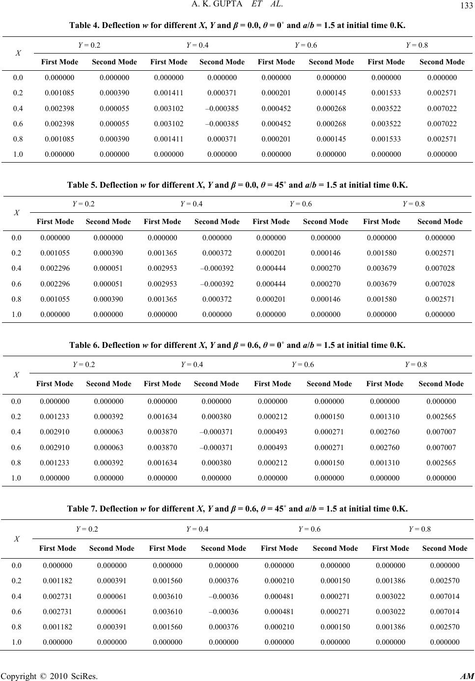

A. K. GUPTA ET AL.
133
Table 4. Deflection w for different X, Y and β = 0.0, θ = 0˚ and a/b = 1.5 at initial time 0.K.
Y = 0.2 Y = 0.4 Y = 0.6 Y = 0.8
X
First Mode Second Mode First ModeSecond ModeFirst ModeSecond ModeFirst Mode Second Mode
0.0 0.000000 0.000000 0.000000 0.000000 0.000000 0.000000 0.000000 0.000000
0.2 0.001085 0.000390 0.001411 0.000371 0.000201 0.000145 0.001533 0.002571
0.4 0.002398 0.000055 0.003102 –0.000385 0.000452 0.000268 0.003522 0.007022
0.6 0.002398 0.000055 0.003102 –0.000385 0.000452 0.000268 0.003522 0.007022
0.8 0.001085 0.000390 0.001411 0.000371 0.000201 0.000145 0.001533 0.002571
1.0 0.000000 0.000000 0.000000 0.000000 0.000000 0.000000 0.000000 0.000000
Table 5. Deflection w for different X, Y and β = 0.0, θ = 45˚ and a/b = 1.5 at initial time 0.K.
Y = 0.2 Y = 0.4 Y = 0.6 Y = 0.8
X
First Mode Second Mode First Mode Second ModeFirst ModeSecond ModeFirst Mode Second Mode
0.0 0.000000 0.000000 0.000000 0.000000 0.000000 0.000000 0.000000 0.000000
0.2 0.001055 0.000390 0.001365 0.000372 0.000201 0.000146 0.001580 0.002571
0.4 0.002296 0.000051 0.002953 –0.000392 0.000444 0.000270 0.003679 0.007028
0.6 0.002296 0.000051 0.002953 –0.000392 0.000444 0.000270 0.003679 0.007028
0.8 0.001055 0.000390 0.001365 0.000372 0.000201 0.000146 0.001580 0.002571
1.0 0.000000 0.000000 0.000000 0.000000 0.000000 0.000000 0.000000 0.000000
Table 6. Deflection w for different X, Y and β = 0.6, θ = 0˚ and a/b = 1.5 at initial time 0.K.
Y = 0.2 Y = 0.4 Y = 0.6 Y = 0.8
X
First Mode Second Mode First Mode Second ModeFirst ModeSecond ModeFirst Mode Second Mode
0.0 0.000000 0.000000 0.000000 0.000000 0.000000 0.000000 0.000000 0.000000
0.2 0.001233 0.000392 0.001634 0.000380 0.000212 0.000150 0.001310 0.002565
0.4 0.002910 0.000063 0.003870 –0.000371 0.000493 0.000271 0.002760 0.007007
0.6 0.002910 0.000063 0.003870 –0.000371 0.000493 0.000271 0.002760 0.007007
0.8 0.001233 0.000392 0.001634 0.000380 0.000212 0.000150 0.001310 0.002565
1.0 0.000000 0.000000 0.000000 0.000000 0.000000 0.000000 0.000000 0.000000
Table 7. Deflection w for different X, Y and β = 0.6, θ = 45˚ and a/b = 1.5 at initial time 0.K.
Y = 0.2 Y = 0.4 Y = 0.6 Y = 0.8
X
First Mode Second Mode First Mode Second ModeFirst ModeSecond Mode First Mode Second Mode
0.0 0.000000 0.000000 0.000000 0.000000 0.000000 0.000000 0.000000 0.000000
0.2 0.001182 0.000391 0.001560 0.000376 0.000210 0.000150 0.001386 0.002570
0.4 0.002731 0.000061 0.003610 –0.00036 0.000481 0.000271 0.003022 0.007014
0.6 0.002731 0.000061 0.003610 –0.00036 0.000481 0.000271 0.003022 0.007014
0.8 0.001182 0.000391 0.001560 0.000376 0.000210 0.000150 0.001386 0.002570
1.0 0.000000 0.000000 0.000000 0.000000 0.000000 0.000000 0.000000 0.000000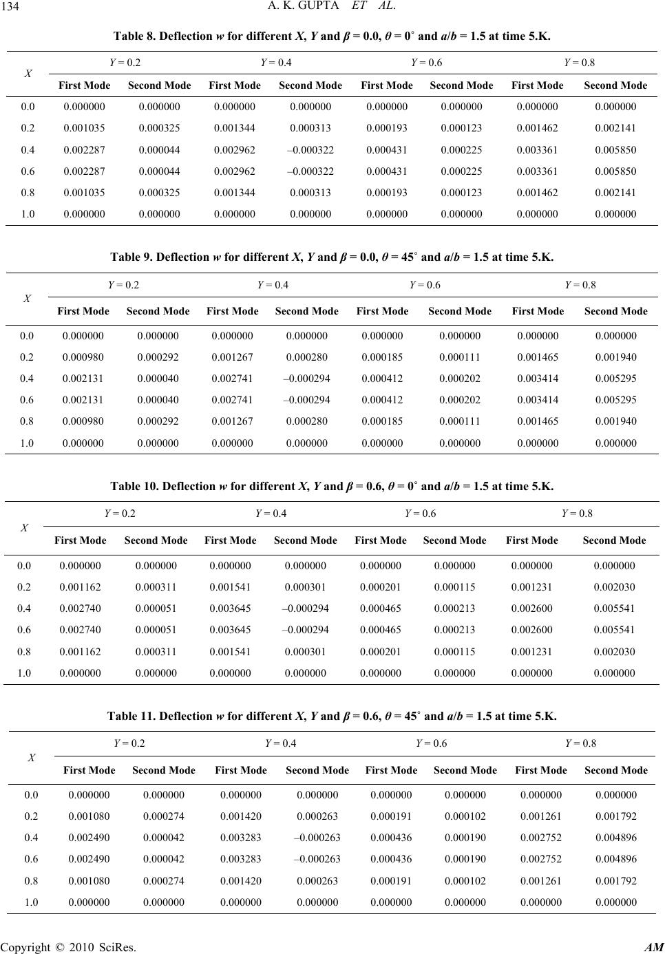

A. K. GUPTA ET AL.
134
Table 8. Deflection w for different X, Y and β = 0.0, θ = 0˚ and a/b = 1.5 at time 5.K.
Y = 0.2 Y = 0.4 Y = 0.6 Y = 0.8
X
First Mode Second Mode First ModeSecond ModeFirst ModeSecond ModeFirst Mode Second Mode
0.0 0.000000 0.000000 0.000000 0.000000 0.000000 0.000000 0.000000 0.000000
0.2 0.001035 0.000325 0.001344 0.000313 0.000193 0.000123 0.001462 0.002141
0.4 0.002287 0.000044 0.002962 –0.000322 0.000431 0.000225 0.003361 0.005850
0.6 0.002287 0.000044 0.002962 –0.000322 0.000431 0.000225 0.003361 0.005850
0.8 0.001035 0.000325 0.001344 0.000313 0.000193 0.000123 0.001462 0.002141
1.0 0.000000 0.000000 0.000000 0.000000 0.000000 0.000000 0.000000 0.000000
Table 9. Deflection w for different X, Y and β = 0.0, θ = 45˚ and a/b = 1.5 at time 5.K.
Y = 0.2 Y = 0.4 Y = 0.6 Y = 0.8
X
First Mode Second Mode First Mode Second ModeFirst ModeSecond ModeFirst Mode Second Mode
0.0 0.000000 0.000000 0.000000 0.000000 0.000000 0.000000 0.000000 0.000000
0.2 0.000980 0.000292 0.001267 0.000280 0.000185 0.000111 0.001465 0.001940
0.4 0.002131 0.000040 0.002741 –0.000294 0.000412 0.000202 0.003414 0.005295
0.6 0.002131 0.000040 0.002741 –0.000294 0.000412 0.000202 0.003414 0.005295
0.8 0.000980 0.000292 0.001267 0.000280 0.000185 0.000111 0.001465 0.001940
1.0 0.000000 0.000000 0.000000 0.000000 0.000000 0.000000 0.000000 0.000000
Table 10. Deflection w for different X, Y and β = 0.6, θ = 0˚ and a/b = 1.5 at time 5.K.
Y = 0.2 Y = 0.4 Y = 0.6 Y = 0.8
X
First Mode Second Mode First Mode Second ModeFirst ModeSecond ModeFirst Mode Second Mode
0.0 0.000000 0.000000 0.000000 0.000000 0.000000 0.000000 0.000000 0.000000
0.2 0.001162 0.000311 0.001541 0.000301 0.000201 0.000115 0.001231 0.002030
0.4 0.002740 0.000051 0.003645 –0.000294 0.000465 0.000213 0.002600 0.005541
0.6 0.002740 0.000051 0.003645 –0.000294 0.000465 0.000213 0.002600 0.005541
0.8 0.001162 0.000311 0.001541 0.000301 0.000201 0.000115 0.001231 0.002030
1.0 0.000000 0.000000 0.000000 0.000000 0.000000 0.000000 0.000000 0.000000
Table 11. Deflection w for different X, Y and β = 0.6, θ = 45˚ and a/b = 1.5 at time 5.K.
Y = 0.2 Y = 0.4 Y = 0.6 Y = 0.8
X
First Mode Second Mode First ModeSecond ModeFirst ModeSecond ModeFirst Mode Second Mode
0.0 0.000000 0.000000 0.000000 0.000000 0.000000 0.000000 0.000000 0.000000
0.2 0.001080 0.000274 0.001420 0.000263 0.000191 0.000102 0.001261 0.001792
0.4 0.002490 0.000042 0.003283 –0.000263 0.000436 0.000190 0.002752 0.004896
0.6 0.002490 0.000042 0.003283 –0.000263 0.000436 0.000190 0.002752 0.004896
0.8 0.001080 0.000274 0.001420 0.000263 0.000191 0.000102 0.001261 0.001792
1.0 0.000000 0.000000 0.000000 0.000000 0.000000 0.000000 0.000000 0.000000

A. K. GUPTA ET AL.
135
On comparison with [13], it is concluded that:
Time period K is more for non-uniform thickness in
case of parabolic variation as comparison to linear varia-
tion.
Deflection w is less for non-uniform thickness in case
of parabolic variation as comparison to linear variation.
In this way, authors concluded that parabolic variation
is more useful than linear variation.
7. References
[1] M. S. Dhotarad and N. Ganesan, “Vibration Analysis of a
Rectangular Plate Subjected to a Thermal Gradient,” Jour-
nal of Sound and Vibration, Vol. 60, No. 4, 1978, pp.
481-497.
[2] M. Amabili and R. Garziera, “Transverse Vibrations of
Circular, Annular Plates with Several Combinations of
Boundary Conditions,” Journal of Sound and Vibration,
Vol. 228, No. 2, 1999, pp. 443-446.
[3] S. Ceribasi and G. Altay, “Free Vibration of Super Ellip-
tical Plates with Constant and Variable Thickness by Ritz
Method,” Journal of Sound and Vibration, Vol. 319, No.
1-2, 2009, pp. 668-680.
[4] U. S. Gupta, A. H. Ansari and S. Sharma, “Vibration
Analysis of Non-Homogenous Circular Plate of Non-
Linear Thickness Variation by Differential Quadrature
Method,” Journal of Sound and Vibration, Vol. 298, No.
4-5, 2006, pp. 892-906.
[5] R. K. Jain and S. R. Soni, “Free Vibrations of Rectangu-
lar Plates of Parabolically Varying Thicknesses,” Indian
Journal of Pure and Applied Mathematics, Vol. 4, No. 3,
1973, pp. 267-277.
[6] B. Singh and V. Saxena, “Transverse Vibration of Rec-
tangular Plate with Bidirectional Thickness Variation,”
Journal of Sound and Vibration, Vol. 198, No. 1, 1996,
pp. 51-65.
[7] J. S. Tomar, D. C. Gupta and V. Kumar, “Free Vibrations
of Non-Homogeneous Circular Plate of Variable Thick-
ness Resting on Elastic Foundation,” Journal of Engi-
neering Design, Vol. 1, No. 3, 1983, pp. 49-54.
[8] J. S. Yang, “The Vibration of a Circular Plate with Vary-
ing Thickness,” Journal of Sound and Vibration, Vol. 165,
No. 1, 1993, pp. 178-184.
[9] U. S. Gupta, A. H. Ansari and S. Sharma, “Vibration of
Non-Homogeneous Circular Mindlin Plates with Variable
Thickness,” Journal of Sound and Vibration, Vol. 302,
No. 1-2, 2007, pp. 1-17.
[10] D. V. Bambill, C. A. Rossit, P. A. A. Laura and R. E.
Rossi, “Transverse Vibrations of an Orthotropic Rectan-
gular Plate of Linearly Varying Thickness and with a
Free Edge,” Journal of Sound and Vibration, Vol. 235,
No. 3, 2000, pp. 530-538.
[11] A. W. Leissa, “Recent Research in Plate Vibrations: Clas-
sical Theory,” The Shock and Vibration Digest, Vol. 9,
No. 10, 1977, pp. 13-24.
[12] Z. Sobotka, “Free Vibration of Visco-Elastic Orthotropic
Rectangular Plates,” Acta Technica (Czech Science Ad-
vanced Views), No. 6, 1978, pp. 678-705.
[13] A. K. Gupta, A. Kumar and Y. K. Gupta, “Vibration
Study of Visco-Elastic Parallelogram Plate of Linearly
Varying Thickness,” International Journal of Engineer-
ing and Interdisciplinary Mathematics, accepted for pub-
lication.
[14] K. Nagaya, “Vibrations and Dynamic Response of Vis-
coelastic Plates on Non-Periodic Elastic Supports,” Jour-
nal of Engineering for Industry, Vol. 99, 1977, pp. 404-409.

A. K. GUPTA ET AL.
136
Appendix: List of Symbols
a length of the plate, ň Visco-elastic constants,
b width of the plate, w(ξ, η ,t) deflection of the plate i.e. amplitude,
ξ and η co-ordinates in the plane of the plate, W(ξ,η) deflection function,
h thickness of the plate at the point (ξ, η), T(t) time function,
E young’s modulus, β taper constant,
G shear modulus, K time period,
ν Poisson’s ratio, h
0 h at ξ = 0,
D
~
visco-elastic operator, a/b aspect ratio,
D Eh3/12(1-ν2), flexural rigidity, θ skew angle,
T
max Kinetic energy,
ρ mass density per unit volume of the
plate material, V Strain energy,
t time, λ2 12ρ (1-ν2)a4/Eh0
2, a frequency parameter