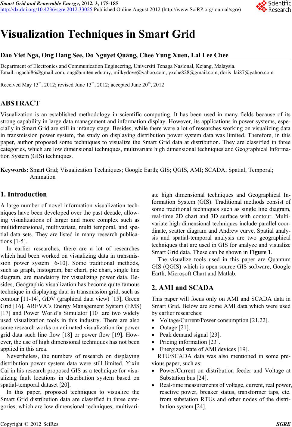
Smart Grid and Renewable Energy, 2012, 3, 175-185
http://dx.doi.org/10.4236/sgre.2012.33025 Published Online August 2012 (http://www.SciRP.org/journal/sgre) 175
Visualization Techniques in Smart Grid
Dao Viet Nga, Ong Hang See, Do Nguyet Quang, Chee Yung Xuen, Lai Lee Chee
Department of Electronics and Communication Engineering, Universiti Tenaga Nasional, Kejang, Malaysia.
Received May 13th, 2012; revised June 13th, 2012; accepted June 20th, 2012
ABSTRACT
Visualization is an established methodology in scientific computing. It has been used in many fields because of its
strong capability in large data manage ment and information display. However, its applications in power systems, espe-
cially in Smart Grid are still in infancy stag e. Besides, while there were a lot of researches working on visualizing data
in transmission power system, the study on displaying distribution power system data was limited. Therefore, in this
paper, author proposed some techniques to visualize the Smart Grid data at distribution. They are classified in three
categories, which are low dimensional techniques, multivariate high dimensional techn iques and Geograph ical Informa-
tion System (GIS) techniques.
Keywords: Smart Grid; Visualization Techniques; Google Earth; GIS; QGIS, AMI; SCADA; Spatial; Temporal;
Animation
1. Introduction
A large number of novel information visualization tech-
niques have been developed over the past decade, allow-
ing visualizations of larger and more complex such as
multidimensional, multivariate, multi temporal, and spa-
tial data sets. They are listed in many research publica-
tions [1-5].
In earlier researches, there are a lot of researches
which had been worked on visualizing data in transmis-
sion power system [6-10]. Some traditional methods,
such as graph, histogram, bar chart, pie chart, single line
diagram, are mandatory for visualizing power data. Be-
sides, Geographic visualization has become quite famous
technique in displaying data in transmission grid, such as
contour [11-14], GDV (graphical data view) [15], Green
Grid [16]. AREVA’s Energy Management System (EMS)
[17] and Power World’s Simulator [10] are two widely
used visualization tools in this industry. There are also
some research works on animated visualization for power
grid data such line flow [18] or power flow [19]. How-
ever, the use of high dimensional techniques has not been
applied in this area.
Nevertheless, the numbers of research on displaying
distribution power system data were still limited. Yixin
Cai in his research proposed GIS as a technique for visu-
alizing fault locations in distribution system based on
spatial-temporal dataset [20].
In this paper, proposed techniques to visualize the
Smart Grid distribution data are classified in three cate-
gories, which are low dimensional techniques, multivari-
ate high dimensional techniques and Geographical In-
formation System (GIS). Traditional methods consist of
some traditional techniques such as single line diagram,
real-time 2D chart and 3D surface with contour. Multi-
variate high dimensional techniques include parallel coor-
dinate, scatter diagram and Andrew curve. Spatial analy-
sis and spatial-temporal analysis are two geographical
techniques that are used in GIS for analyze and visualize
Smart Grid data. These can be shown in Figure 1.
The visualize tools used in this paper are Quantum
GIS (QGIS) which is open source GIS software, Google
Earth, Microsoft Chart and Matlab.
2. AMI and SCADA
This paper will focus only on AMI and SCADA data in
Smart Grid. Below are some AMI data which were used
by earlier researches:
 Voltage/Current/Power consumption [21,22].
 Outage [21] .
 Peak demand s i gna l [2 3 ] .
 Pricing information [23].
 Energized state of AMI de vi c es [19].
RTU/SCADA data was also mentioned in some pre-
vious paper, such as:
 Power/Current on distribution feeder and Voltage at
Substation bus [24].
 Real-time measurem ents of vol ta ge, current, real power,
reactive power, breaker status, transformer taps, etc.
from substation RTUs and other nodes of the distri-
bution syst em [24].

Visualization Techniques in Smart Grid
176
This project concentrates on Uniten-TNBR Smart Grid
Testbed. There are 16 substations located in this area
which divided into 3 main substations such as TNB SSU,
TNB SSU1, and TNB SSU2. Each substation is divided
into smaller unit called PE. The detail of AMI and
SCADA network diag ram is shown in Figure 2.
3. Traditional Visualization Techniques
3.1. Single Line Diagram
The operators use single line diagrams to get an overview
of the AMI/SCADA network system. Single line dia-
grams display the interconnection between substations
and some critical parameters such as line status, AMI
energized status. Hence, the diagram allows the operators
to have a macro level view of the system as shown in
Figure 3.
3.2. Real Time 2D Bar Chart
Bar chart is one of traditional techniques to visualize data
in many fields. However, instead of static data, dynamic
data is displayed in form of bar chart. The x-axis repre-
sents number of data points while the y-axis represents
total power consumption of all substations, as shown in
Figure 4. Since a data point was added in every 5 min-
utes and the maximum of point displaying in x-axis are
200, the chart can visualize the changing of total power
consumption over 1000 minutes time interval. When the
new data point adds to the chart, the data at the most left
of the horizontal axis will be removed.
Figure 1. Visualization techniques in Smart Grid.
Figure 2. AMI and SCADA network diagram for Uniten-TNBR smart grid testbed.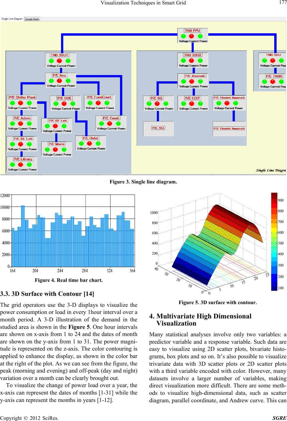

Visualization Techniques in Smart Grid 177
Figure 3. Single line diagram.
Figure 4. Real time bar chart.
3.3. 3D Surface with Contour [14]
The grid operators use the 3-D displays to visualize the
power consumption or load in every 1ho ur interval over a
month period. A 3-D illustration of the demand in the
studied area is shown in the Figure 5. One hour intervals
are shown on x-axis from 1 to 24 and the dates of month
are shown on the y-axis from 1 to 31. The power magni-
tude is represented on the z-axis. The color contouring is
applied to enhance the disp lay, as shown in the color bar
at the right of the plot. As we can see from the figure, the
peak (morning and evening) and off-peak (day and night)
variation over a month can be clearly brought out.
To visualize the change of power load over a year, the
x-axis can represent the dates of months [1-31] while the
y-axis can represent the months in years [1-12].
Figure 5. 3D surface wi th contour.
4. Multivariate High Dimensional
Visualization
Many statistical analyses involve only two variables: a
predictor variable and a response variable. Such data are
easy to visualize using 2D scatter plots, bivariate histo-
grams, box plots and so on. It’s also possible to visualize
trivariate data with 3D scatter plots or 2D scatter plots
with a third variable encoded with color. However, many
datasets involve a larger number of variables, making
direct visualization more difficult. There are some meth-
ods to visualize high-dimensional data, such as scatter
diagram, parallel coordinate, and Andrew curve. This can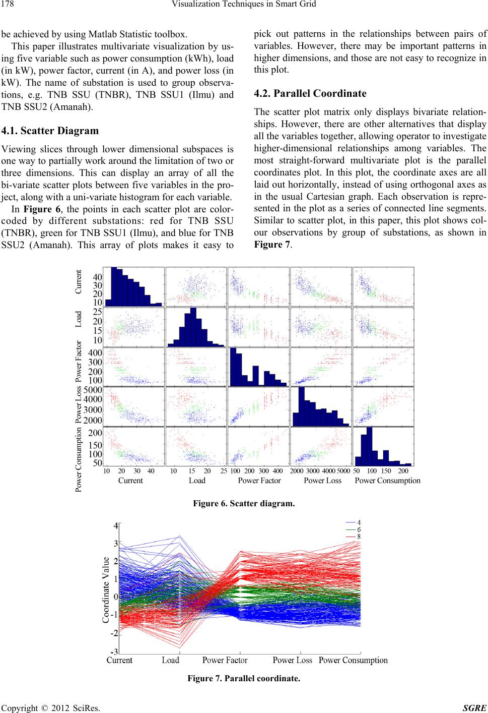

Visualization Techniques in Smart Grid
178
be achieved by using Matlab Statistic toolbox.
This paper illustrates multivariate visualization by us-
ing five variable such as power consumption (kWh), load
(in kW), power factor, current (in A), and power loss (in
kW). The name of substation is used to group observa-
tions, e.g. TNB SSU (TNBR), TNB SSU1 (Ilmu) and
TNB SSU2 (Amanah).
4.1. Scatter Diagram
Viewing slices through lower dimensional subspaces is
one way to partially work around the limitation of two or
three dimensions. This can display an array of all the
bi-variate scatter plots between five variables in the pro-
ject, along with a uni-variate histogram for each variable.
In Figure 6, the points in each scatter plot are color-
coded by different substations: red for TNB SSU
(TNBR), green for TNB SSU1 (Ilmu), and blue for TNB
SSU2 (Amanah). This array of plots makes it easy to
pick out patterns in the relationships between pairs of
variables. However, there may be important patterns in
higher dimensions, and those are not easy to recognize in
this plot.
4.2. Parallel Coordinate
The scatter plot matrix only displays bivariate relation-
ships. However, there are other alternatives that display
all the variables together, allowing op erator to investigate
higher-dimensional relationships among variables. The
most straight-forward multivariate plot is the parallel
coordinates plot. In this plot, the coordinate axes are all
laid out horizontally, instead of using orthogonal axes as
in the usual Cartesian graph. Each observation is repre-
sented in the plot as a series of connected line segments.
Similar to scatter plot, in this paper, this plot shows col-
our observations by group of substations, as shown in
Figure 7.
Figure 6. Scatter diagram.
Figure 7. Parallel coordinate.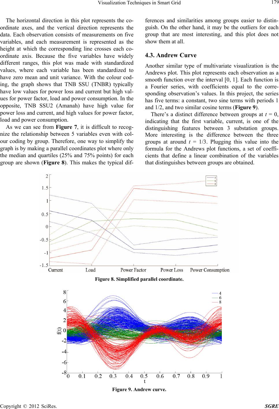

Visualization Techniques in Smart Grid 179
The horizontal direction in this plot represents the co-
ordinate axes, and the vertical direction represents the
data. Each observation consists of measurements on five
variables, and each measurement is represented as the
height at which the corresponding line crosses each co-
ordinate axis. Because the five variables have widely
different ranges, this plot was made with standardized
values, where each variable has been standardized to
have zero mean and unit variance. With the colour cod-
ing, the graph shows that TNB SSU (TNBR) typically
have low values for power loss and current but high val-
ues for power factor, load and power consumption. In the
opposite, TNB SSU2 (Amanah) have high value for
power loss and current, and high values for power factor,
load and power consumption.
As we can see from Figure 7, it is difficult to recog-
nize the relationship between 5 variables even with col-
our coding by group. Therefore, one way to simplify the
graph is by making a parallel coordinates plot where only
the median and quartiles (25% and 75% points) for each
group are shown (Figure 8). This makes the typical dif-
ferences and similarities among groups easier to distin-
guish. On the other hand, it may be the outliers for each
group that are most interesting, and this plot does not
show them at all.
4.3. Andrew Curve
Another similar type of multivariate visualization is the
Andrews plot. This plot represents each observation as a
smooth function over the interval [0, 1]. Each function is
a Fourier series, with coefficients equal to the corre-
sponding observation’s values. In this project, the series
has five terms: a constant, two sine terms with periods 1
and 1/2, and two similar cosine terms (Figure 9).
There’s a distinct difference between groups at t = 0,
indicating that the first variable, current, is one of the
distinguishing features between 3 substation groups.
More interesting is the difference between the three
groups at around t = 1/3. Plugging this value into the
formula for the Andrews plot functions, a set of coeffi-
cients that define a linear combination of the variables
that distinguishes between groups are obtained.
Figure 8. Simplified parallel coordinate.
Figure 9. Andrew curve.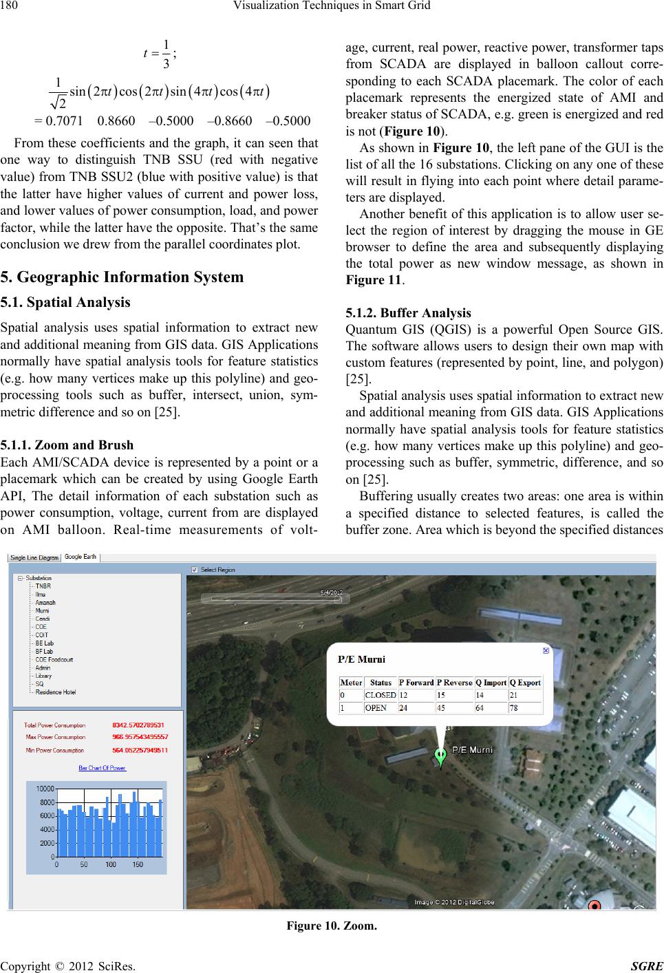

Visualization Techniques in Smart Grid
180
1
3
t;

1sin2cos 2sin 4cos 4
2tttt
= 0.7071 0.8660 –0.5000 –0.8660 –0.5000
From these coefficients and the graph, it can seen that
one way to distinguish TNB SSU (red with negative
value) from TNB SSU2 (blue with positive value) is that
the latter have higher values of current and power loss,
and lower values of power consumption, load, and power
factor, while the latter have the opposite. That’s th e same
conclusio n we d rew from the parallel coo rdinates pl o t .
5. Geographic Information System
5.1. Spatial Analysis
Spatial analysis uses spatial information to extract new
and additional meaning from GIS data. GIS Applications
normally have spatial analysis tools for feature statistics
(e.g. how many vertices make up this polyline) and geo-
processing tools such as buffer, intersect, union, sym-
metric difference and so on [25].
5.1.1. Zoom and Brush
Each AMI/SCADA device is represented by a point or a
placemark which can be created by using Google Earth
API, The detail information of each substation such as
power consumption, voltage, current from are displayed
on AMI balloon. Real-time measurements of volt-
age, current, real power, reactive power, transformer taps
from SCADA are displayed in balloon callout corre-
sponding to each SCADA placemark. The color of each
placemark represents the energized state of AMI and
breaker status of SCADA, e.g. green is energized and red
is not (Figure 10).
As shown in Figure 10, the left pane of the GUI is the
list of all the 16 substations. Clicking on any one of these
will result in flying into each point where detail parame-
ters are displayed.
Another benefit of this application is to allow user se-
lect the region of interest by dragging the mouse in GE
browser to define the area and subsequently displaying
the total power as new window message, as shown in
Figure 11.
5.1.2. Buffer Analysis
Quantum GIS (QGIS) is a powerful Open Source GIS.
The software allows users to design their own map with
custom features (r epresented by point, lin e, and polygon)
[25].
Spatial analysis uses spatial in formation to extract new
and additional meaning from GIS data. GIS Applications
normally have spatial analysis tools for feature statistics
(e.g. how many vertices make up this polyline) and geo-
processing such as buffer, symmetric, difference, and so
on [25].
Buffering usually creates two areas: one area is within
a specified distance to selected features, is called the
buffer zone. Area which is beyond the specified distances
Figure 10. Zoom.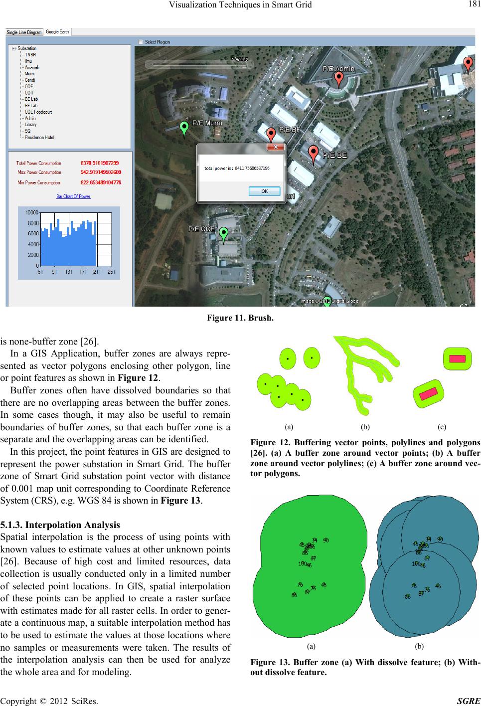

Visualization Techniques in Smart Grid 181
Figure 11. Brush.
is none-buffer zone [26].
In a GIS Application, buffer zones are always repre-
sented as vector polygons enclosing other polygon, line
or point features as shown in Figure 12.
Buffer zones often have dissolved boundaries so that
there are no overlapping areas between the buffer zones.
In some cases though, it may also be useful to remain
boundaries of buffer zones, so that each buffer zone is a
separate and the overlapping areas can be identified.
In this project, the point features in GIS are designed to
represent the power substation in Smart Grid. The buffer
zone of Smart Grid substation point vector with distance
of 0.001 map unit corresponding to Coordinate Reference
System (CRS ), e.g. WGS 84 is shown in Figure 13.
5.1.3. Interpolation Analysis
Spatial interpolation is the process of using points with
known values to estimate values at other unknown points
[26]. Because of high cost and limited resources, data
collection is usually conducted only in a limited number
of selected point locations. In GIS, spatial interpolation
of these points can be applied to create a raster surface
with estimates made for all raster cells. In order to gener-
ate a continuous map, a suitable interpolation method has
to be used to estimate the values at those locations where
no samples or measurements were taken. The results of
the interpolation analysis can then be used for analyze
the whole area and for modeling.
(a) (b) (c)
Figure 12. Buffering vector points, polylines and polygons
[26]. (a) A buffer zone around vector points; (b) A buffer
zone around vector polylines; (c ) A buffer zone around vec-
tor polygons.
(a) (b)
Figure 13. Buffer zone (a) With dissolve feature; (b) With-
out dissolve feature.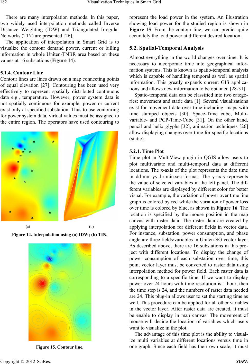

Visualization Techniques in Smart Grid
182
There are many interpolation methods. In this paper,
two widely used interpolation methods called Inverse
Distance Weighting (IDW) and Triangulated Irregular
Networks (TIN) are presented [26].
The application of interpolation in Smart Grid is to
visualize the contour demand power, current or billing
information in whole Uniten-TNBR area based on these
values at 16 substations (Figure 14).
5.1.4. Contour Line
Contour lines are lines drawn on a map connecting points
of equal elevation [27]. Contouring has been used very
effectively to represent spatially distributed continuous
data e.g., temperature. However, power system data is
not spatially continuous for example, power or current
exist only at specified substation. Thus to use contouring
for power system data, virtual values must be assigned to
the entire region. The operators have used contouring to
(a) (b)
Figure 14. Interpolation using (a) IDW; (b) TIN.
Figure 15. Contour line.
represent the load power in the system. An illustration
showing load power for the studied region is shown in
Figure 15. From the contour line, we can predict quite
accurately the load power at different desired location.
5.2. Spatial-Temporal Analysis
Almost everything in the world changes over time. It is
necessary to incorporate time into geographical infor-
mation systems. This is known as spatio-temporal analysis
which is capable of handling temporal as well as spatial
information. This greatly expands current GIS applica-
tions and allows new information to be obtained [28-31].
Spatio-temporal data can be classified into two catego-
ries: movement and static data [1]. Several visualisations
exist for movement data over time including: maps with
time stamped objects [30], Space-Time cube, Multi-
variable- and PCP-Time-Cube [31]. On the other hand,
pencil and helix glyphs [32], animation techniques [26]
allow displaying changes over time for specific locations
(static).
5.2.1. Time Plot
Time plot in MultiView plugin in QGIS allow users to
plot multivariate and multi-temporal data at different
locations. The x-axis of the plot represents the date time
in dd-mm-yy hr:min:sec format. The y-axis represents
the value of selected variables in the left panel. The dif-
ferent variables are displayed by different color for better
visual. For example, the variation of power over time line
graph is colored by red while the variation of power loss
over time is colored by blue, as shown in Figure 16. The
location is specified by the mouse position in the map
canvas with raster data. The raster data are created by
applying interpolation for different fields in vector data.
For instance, substation, power consumption, and phase
angle are three fields/variables in Uniten-SG vector layer.
As described above, there are 16 substations in this pro-
ject with different locations. To display the change of
power consumption of each substation over time, this
point vector layer must be converted to raster data using
interpolation method for power field. Each raster data is
corresponding to a specific time. If we want to display
power over 24 hours with time resolution is 1 hour, then
the time step is 24, and the numbers of raster data needed
are 24. This plug-in allows user to set the starting time as
well. This proced ure c an b e applied for all other variables
in the vector layer. After raster data are created, it must
be enable to display in map canvas. The movement of
mouse will decide the location of variables which users
want to visualize in the plot.
The advantage o f this time plot is the ability to v isual-
ize multi variables at different locations versus time in
one graph. Since each field has their own scale, it must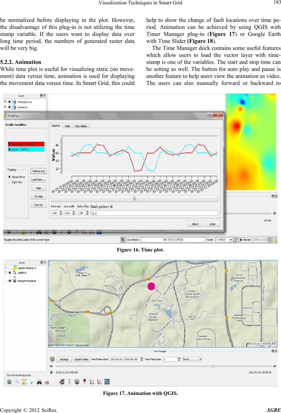

Visualization Techniques in Smart Grid
183
be normalized before displaying in the plot. However,
the disadvantage of this plug-in is not utilizing the time
stamp variable. If the users want to display data over
long time period, the numbers of generated raster data
will be very big.
help to show the change of fault locations over time pe-
riod. Animation can be achieved by using QGIS with
Timer Manager plug-in (Figure 17) or Google Earth
with Time Slider (Figure 18).
The Time Manager dock contains some useful features
which allow users to load the vector layer with time-
stamp is one of the variables. The start and stop time can
be setting as well. The button for auto play and pause is
another feature to help users view the animation as video.
The users can also manually forward or backward to
5.2.2. Animation
While time plot is useful for visualizing static (no move-
ment) data versus time, animation is used for displaying
the movement data versus time. In Smart Grid, this could
Figure 16. Time plot.
Figure 17. Animation with QGIS.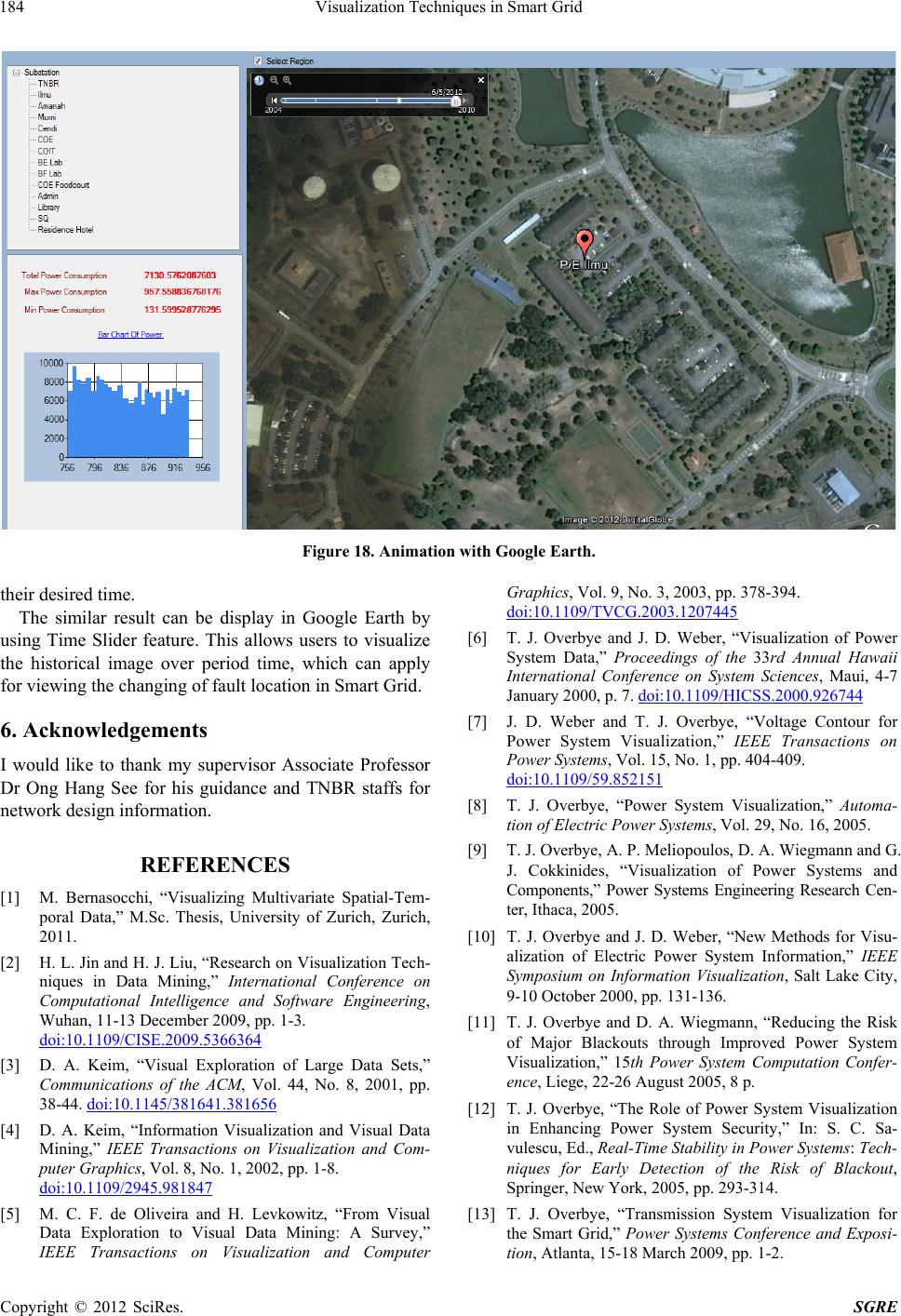

Visualization Techniques in Smart Grid
184
Figure 18. Animation with Google Earth.
their desired time.
The similar result can be display in Google Earth by
using Time Slider feature. This allows users to visualize
the historical image over period time, which can apply
for viewing the changing of fault location in Smart Grid.
6. Acknowledgements
I would like to thank my supervisor Associate Professor
Dr Ong Hang See for his guidance and TNBR staffs for
network design inf ormation.
REFERENCES
[1] M. Bernasocchi, “Visualizing Multivariate Spatial-Tem-
poral Data,” M.Sc. Thesis, University of Zurich, Zurich,
2011.
[2] H. L. Jin and H. J. Liu, “Research on Visualization Tech-
niques in Data Mining,” International Conference on
Computational Intelligence and Software Engineering,
Wuhan, 11-13 December 2009, pp. 1-3.
doi:10.1109/CISE.2009.5366364
[3] D. A. Keim, “Visual Exploration of Large Data Sets,”
Communications of the ACM, Vol. 44, No. 8, 2001, pp.
38-44. doi:10.1145/381641.381656
[4] D. A. Keim, “Information Visualization and Visual Data
Mining,” IEEE Transactions on Visualization and Com-
puter Graphics, Vol. 8, No. 1, 2002, pp. 1-8.
doi:10.1109/2945.981847
[5] M. C. F. de Oliveira and H. Levkowitz, “From Visual
Data Exploration to Visual Data Mining: A Survey,”
IEEE Transactions on Visualization and Computer
Graphics, Vol. 9, No. 3, 2003, pp. 378-394.
doi:10.1109/TVCG.2003.1207445
[6] T. J. Overbye and J. D. Weber, “Visualization of Power
System Data,” Proceedings of the 33rd Annual Hawaii
International Conference on System Sciences, Maui, 4-7
January 2000, p. 7. doi:10.1109/HICSS.2000.926744
[7] J. D. Weber and T. J. Overbye, “Voltage Contour for
Power System Visualization,” IEEE Transactions on
Power Systems, Vol. 15, No. 1, pp. 404-409.
doi:10.1109/59.852151
[8] T. J. Overbye, “Power System Visualization,” Automa-
tion of Electric Power Systems, Vol. 29, No. 16, 2005.
[9] T. J. Overbye, A. P. Meliopoulos, D. A. Wiegmann and G.
J. Cokkinides, “Visualization of Power Systems and
Components,” Power Systems Engineering Research Cen-
ter, Ithaca, 2005.
[10] T. J. Overbye and J. D. Weber, “New Methods for Visu-
alization of Electric Power System Information,” IEEE
Symposium on Information Visualization, Salt Lake City,
9-10 October 2000, pp. 131-136.
[11] T. J. Overbye and D. A. Wiegmann, “Reducing the Risk
of Major Blackouts through Improved Power System
Visualization,” 15th Power System Computation Confer-
ence, Liege, 22-26 August 2005, 8 p.
[12] T. J. Overbye, “The Role of Power System Visualization
in Enhancing Power System Security,” In: S. C. Sa-
vulescu, Ed., Real-Time Stability in Power Systems: Tech-
niques for Early Detection of the Risk of Blackout,
Springer, New York, 2005, pp. 293-314.
[13] T. J. Overbye, “Transmission System Visualization for
the Smart Grid,” Power Systems Conference and Exposi-
tion, Atlanta, 15-18 March 2009, pp. 1-2.

Visualization Techniques in Smart Grid 185
[14] R. Klump, D. Schooley and T. Overbye, “An Advanced
Visualization Platform for Real-Time Simulations,” 14th
Power System Computation Conference, Sevilla, 24-28
June 2002, 8 p.
[15] T. J. Overbye, E. M. Rantanen and S. Judd, “Electric
Power Control Center Visualization Using Geographic
Data Views,” Bulk Power System Dynamics and Con-
trol—VII. Revitalizing Operational Reliability, 2007 iREP
Symposium, Charleston, 19-24 August 2007, pp. 1-8.
doi:10.1109/TVCG.2008.197
[16] P. C. Wong, K. Schneider, P. Mackey, H. Foote, G. Chin,
R. Guttromson and J. Thomas, “A Novel Visualization
Technique for Electric Power Grid Analytics,” IEEE
Transactions on Visualization and Computer Graphics,
Vol. 15, No. 3, 2009, pp. 410-423.
[17] AREVA T & D Energy Management Systems, 2008.
Available from: http://www.areva-td.com
[18] Y. Sun and T. J. Overbye, “Visualization for Power Sys-
tem Contingency Analysis Data,” IEEE Transactions on
Power Systems, Vol. 19, No. 4, 2004, pp. 1859-1866.
doi:10.1109/TPWRS.2004.836193
[19] E. Boardman, “The Role of Integrated Distribution Man-
agement Systems in Smart Grid Implementations,” Power
and Energy Society General Meeting, Minneapolis, 25-29
July 2010, pp. 1-6.
[20] Y. X. Cai and M.-Y. Chow, “Exploratory Analysis of
Massive Data for Distribution Fault Diagnosis in Smart
Grids,” Power & Energy Society General Meeting, Cal-
gary, 26-30 July 2009, pp. 1-6.
doi:10.1109/PES.2009.5275689
[21] H. Tram, “Technical and Operation Considerations in
Using Smart Metering for Outage Management,” Trans-
mission and Distribution Conference and Exposition,
Chicago, 21-24 April 2008, pp. 1-3.
doi:10.1109/TDC.2008.4517273
[22] J. Triplett, S. Rinell and J. Foote, “Evaluating Distribu-
tion System Losses Using Data from Deployed AMI and
GIS Systems,” Rural Electric Power Conference, Or-
lando, 16-19 May 2010, pp. C1-C8.
doi:10.1109/REPCON.2010.5476204
[23] D. Y. R. Nagesh, J. V. V. Krishna and S. S. Tulasiram,
“A Real-Time Architecture for Smart Energy Manage-
ment,” Innovative Smart Grid Technologies, Gaithersburg,
19-21 January 2010, pp. 1-4.
[24] S. Nunoo and A. K. Ofei, “Distribution Automation (DA)
Using Supervisory Control and Data Acquisition (SCADA)
with Advanced Metering Infrastructure (AMI),” 2010
IEEE Conference on Innovative Technologies for an Effi-
cient and Reliable Electricity Supply, Waltham, 27-29
September 2010, pp. 454-458.
doi:10.1109/CITRES.2010.5619797
[25] D. J. Maguire, M. Batty and M. F. Goodchild, “GIS, Spa-
tial Analysis, and Modelling,” ESRI Press, Redlands,
2005.
[26] T. Sutton, O. Dassau and M. Sutton, “A Gentle Introduc-
tion to GIS,” Chief Directorate: Spatial Planning & In-
formation, Eastern Cape, 2009.
[27] http://raider.mountunion.edu/~mcnaugma/topographic%2
0maps/contour.htm
[28] P. Compieta, S. Di Martino, M. Bertolotto, F. Ferrucci
and T. Kechadi, “Exploratory Spatio-Temporal Data Min-
ing and Visualization,” Journal of Visual Languages &
Computing, Vol. 18, No. 3, 2007, pp. 255-279.
doi:10.1016/j.jvlc.2007.02.006
[29] M. Weber, M. Alexa and W. Muller, “Visualizing Time-
Series on Spirals,” 2001 IEEE Symposium on Information
Visualization, San Diego, 22-23 October 2001, pp. 7-13.
doi:10.1109/INFVIS.2001.963273
[30] A. Kjellin, L. W. Pettersson, S. Seipel and M. Lind,
“Evaluating 2D and 3D Visualizations of Spatiotemporal
Information,” ACM Transactions on Applied Perception,
Vol. 7, No. 3, 2010, Article ID: 19.
[31] X. Li and M.-J. Kraak, “New Views on Multivariable
Spatiotemporal Data: The Space Time Cube Expanded,”
International Symposium on Spatio-Temporal Modeling,
Spatial Reasoning, Analysis, Data Mining and Data Fu-
sion, Vol. 36, 2005, pp. 199-201.
[32] C. Tominski, P. Schulze-Wollgast and H. Schumann, “3D
Information Visualization for Time Dependent Data on
Maps,” Proceedings of the 9th International Conference
Information Visualization, Cambridge, 6-8 July 2005, pp.
175-181. doi:10.1109/IV.2005.3