Journal of Modern Physics
Vol.4 No.8A(2013), Article ID:36688,17 pages DOI:10.4236/jmp.2013.48A022
The Mathematical Foundations of General Relativity Revisited
CERMICS, Ecole des Ponts ParisTech, Marne-la-Vall_ee Cedex 02, France
Email: jean-francois.pommaret@wanadoo.fr, pommaret@cermics.enpc.fr
Copyright © 2013 Jean-Francois Pommaret. This is an open access article distributed under the Creative Commons Attribution License, which permits unrestricted use, distribution, and reproduction in any medium, provided the original work is properly cited.
Received May 13, 2013; revised June 19, 2013; accepted July 29, 2013
Keywords: General Relativity; Riemann Tensor; Weyl Tensor; Ricci Tensor; Einstein Equations; Lie Groups; Lie Pseudogroups; Differential Sequence; Spencer Operator; Janet Sequence; Spencer Sequence; Differential Module; Homological Algebra; Extension Modules; Split Exact Sequence
ABSTRACT
The purpose of this paper is to present for the first time an elementary summary of a few recent results obtained through the application of the formal theory of partial differential equations and Lie pseudogroups in order to revisit the mathematical foundations of general relativity. Other engineering examples (control theory, elasticity theory, electromagnetism) will also be considered in order to illustrate the three fundamental results that we shall provide successively. 1) VESSIOT VERSUS CARTAN: The quadratic terms appearing in the “Riemann tensor” according to the “Vessiot structure equations” must not be identified with the quadratic terms appearing in the well known “Cartan structure equations” for Lie groups. In particular, “curvature + torsion” (Cartan) must not be considered as a generalization of “curvature alone” (Vessiot). 2) JANET VERSUS SPENCER: The “Ricci tensor” only depends on the nonlinear transformations (called “elations” by Cartan in 1922) that describe the “difference” existing between the Weyl group (10 parameters of the Poincaré subgroup + 1 dilatation) and the conformal group of space-time (15 parameters). It can be defined without using the indices leading to the standard contraction or trace of the Riemann tensor. Meanwhile, we shall obtain the number of components of the Riemann and Weyl tensors without any combinatoric argument on the exchange of indices. Accordingly and contrary to the “Janet sequence”, the “Spencer sequence” for the conformal Killing system and its formal adjoint fully describe the Cosserat equations, Maxwell equations and Weyl equations but General Relativity is not coherent with this result. 3) ALGEBRA VERSUS GEOMETRY: Using the powerful methods of “Algebraic Analysis”, that is a mixture of homological agebra and differential geometry, we shall prove that, contrary to other equations of physics (Cauchy equations, Cosserat equations, Maxwell equations), the Einstein equations cannot be “parametrized”, that is the generic solution cannot be expressed by means of the derivatives of a certain number of arbitrary potential-like functions, solving therefore negatively a 1000 $ challenge proposed by J. Wheeler in 1970. Accordingly, the mathematical foundations of electromagnetism and gravitation must be revisited within this formal framework, though striking it may look like. We insist on the fact that the arguments presented are of a purely mathematical nature and are thus unavoidable.
1. Introduction
The purpose of this paper is to present an elementary summary of a few recent results obtained through the application of the formal theory of systems of ordinary differential (OD) or partial differential (PD) equations and Lie pseudogroups in order to revisit the mathematical foundations of general relativity (GR). More elementary engineering examples (elasticity theory, electromagnetism (EM)) will also be considered in order to illustrate the quoted three fundamental results that we shall provide. The paper, based on the material of two lectures given at the department of mathematics of the university of Montpellier 2, France, in may 2013 and Firenze, Italy, in june 2013, is divided into three parts corresponding to the different formal methods used.
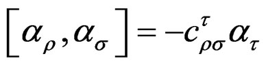
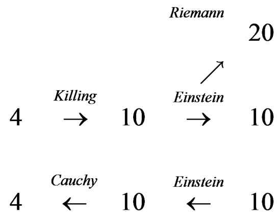
PART 1: In 1880 S. Lie (1842-1899) studied the groups of transformations depending on a finite number of parameters and now called Lie groups of transformations. Ten years later he discovered that these groups are only examples of groups of transformations solutions of linear or nonlinear systems of ordinary differential (OD) or partial differential (PD) equations which may even be of high order and are now called Lie pseudogroups of transformations. During the next fifty years the latter groups have only been studied by two frenchmen, namely Elie Cartan (1869-1951) who is quite famous today, and Ernest Vessiot (1865-1952) who is almost ignored today. We have proved in many books and papers that the Cartan structure equations have nothing to do with the Vessiot structure equations still not known today. Accordingly, the quadratic terms appearing in the Riemann tensor must not be identified with the quadratic terms appearing in the well known Maurer-Cartan equations for Lie groups. In particular, curvature + torsion (Cartan) must not be considered as a generalization of curvature alone (Vessiot).
PART 2: Though we consider that the first formal work on systems of PD equations is dating back to Maurice Janet (1888-1983) who introduced as early as in 1920 a differential sequence now called Janet sequence, it is only around 1970 that Donald Spencer (1912-2001) developped, in a quite independent way, the formal theory of systems of PD equations in order to study Lie pseudogroups, exactly like E. Cartan did with exterior systems. However, all the physicists who tried to understand the only book “Lie equations” that he published in 1972 with A. Kumpera, have been stopped by the fact that the examples of the Introduction (Janet sequence) have nothing to do with the core of the book (Spencer sequence). We may say that the work of Cartan is superseded by the use of the canonical Spencer sequence while the work of Vessiot is superseded by the use of the canonical Janet sequence but the link between these two sequences and thus these two works is not known today. Accordingly, the Spencer sequence for the conformal Killing system and its formal adjoint fully describe the Cosserat equations, Maxwell equations and Weyl equations but general relativity (GR) is not coherent with this result because we shall prove that the Ricci tensor only depends on the nonlinear transformations (called elations by Cartan in 1922) that describe the “difference” existing between the Weyl group (10 parameters of the Poincaré subgroup + 1 dilatation) and the conformal group of space-time (15 parameters).
PART 3: At the same time, mixing differential geometry and homological algebra but always supposing that the reader knows a lot about the work of Spencer, V.P. Palamodov (constant coefficients) and M. Kashiwara (variable coefficients) developped “algebraic analysis” in order to study the formal properties of finitely generated differential modules that do not depend on their presentation or even on a corresponding differential resolution, namely the algebraic analogue of a differential sequence. Using double duality theory, we prove that, contrary to other equations of physics (Cauchy equations, Cosserat equations, Maxwell equations), the Einstein equations cannot be “parametrized”, that is the generic solution cannot be expressed by means of the derivatives of a certain number of arbitrary potential-like functions, solving therefore negatively a 1000 $ challenge proposed by J. Wheeler in 1970.
The new methods involve tools from differential geometry (jet theory, Spencer operator, ![]() -cohomology) and homological algebra (diagram chasing, snake theorem, extension modules, double duality). The reader may just have a look to the book [1] (review in Zbl 1079. 93001) in order to understand the amount of mathematics needed from many domains.
-cohomology) and homological algebra (diagram chasing, snake theorem, extension modules, double duality). The reader may just have a look to the book [1] (review in Zbl 1079. 93001) in order to understand the amount of mathematics needed from many domains.
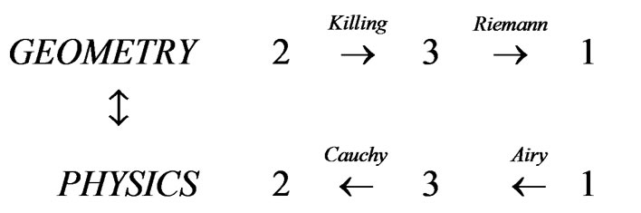
The following diagram summarizes at the same time the historical background and the difficulties presented in the introduction:
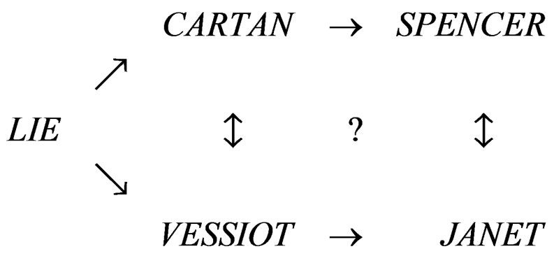
Roughly, Cartan and followers have not been able to “quotient down to the base manifold” [2,3], a result only obtained by Spencer in 1970 through the nonlinear Spencer sequence [4-7] but in a way quite different from the one followed by Vessiot in 1903 for the same purpose [8,9]. Accordingly, the mathematical foundations of mathematical physics must be revisited within this formal framework, though striking it may look like for certain apparently well established theories such as EM (J. C. Maxwell, 1864) and GR (A. Einstein, 1915).
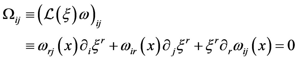
2. First Part: From Lie Groups to Lie Pseudogroups
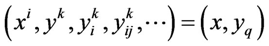
If  is a manifold with local coordinates
 ![]() for
for
 , let
, let ![]() be a fibered manifold over
be a fibered manifold over
 , that is a manifold with local coordinates
  for
for  and
and  simply denoted by
 , projection
and changes of local coordinates
 .
.
If ![]() and
and  are two fibered manifolds over
  with respective local coordinates
  and
and , we denote by
  the fibered product of
 ![]() and
and  over
over  as the new fibered manifold over
  with local coordinates
 . We denote by
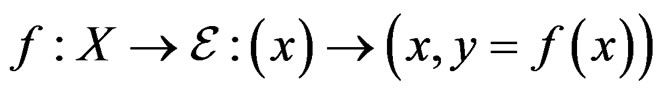
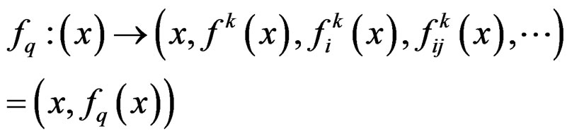
a global section of![]() , that is a map such that
, that is a map such that  but local sections over an open set
  may also be considered when needed. We shall use for simplicity the same notation for a fibered manifold and its set of sections while setting
 . Under a change of coordinates, a section transforms like
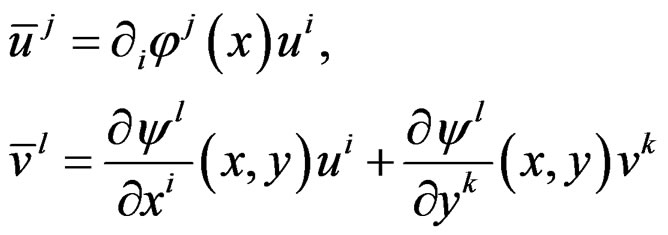
and the derivatives transform like:
 .
.
We may introduce new coordinates  transforming like:
 .
.
We shall denote by  the q-jet bundle of
 ![]()
with local coordinates
called jet coordinates and sections
transforming like the sections
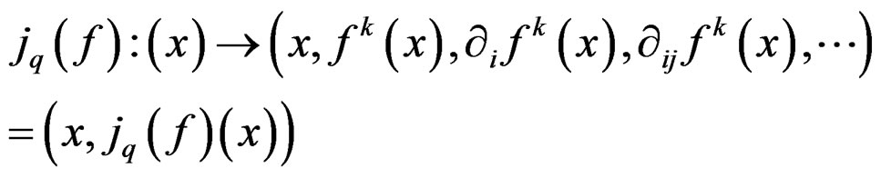
where both  and
and  are over the section
  of
of
![]() . Of course
. Of course  is a fibered manifold over
with projection  while
while  is a fibered manifold over
  with projection
 .
.
DEFINITION 1.1: A (nonlinear) system of order  on
on ![]() is a fibered submanifold
is a fibered submanifold  and a solution of
  is a section
  of
of ![]() such that
such that  is a section of
 .
.
DEFINITION 1.2: When the changes of coordinates have the linear form , we say that
 ![]() is a vector bundle over
is a vector bundle over . Vector bundles will be denoted by capital letters
  and will have sections denoted by
 . In particular, we shall denote as usual by
  the tangent bundle of
 , by
, by
 the cotangent bundle, by
  the bundle of r-forms and by
  the bundle of qsymmetric covariant tensors. When the changes of coordinates have the form
we say that ![]() is an affine bundle over
is an affine bundle over  and we define the associated vector bundle
  over
over  by the local coordinates
  changing like
 . Finally, If
 , we shall denote by
 the open subfibered manifold of
 defined independently of the coordinate system by
  with source projection
and target projection
 .
.
DEFINITION 1.3: If the tangent bundle  has local coordinates
  changing like
 we may introduce the vertical bundle
  as a vector bundle over
 ![]() with local coordinates
with local coordinates  obtained by setting
  and changes
 .
.
Of course, when ![]() is an affine bundle over
is an affine bundle over  with associated vector bundle
  over
over , we have
 .
.
For a later use, if ![]() is a fibered manifold over
is a fibered manifold over  and
and  is a section of
![]() , we denote by
, we denote by  the reciprocal image of
  by
by  as the vector bundle over
  obtained when replacing
  by
by  in each chart. A similar construction may also be done for any affine bundle over
![]() .
.
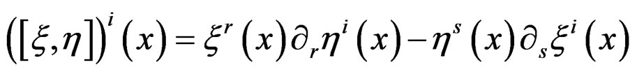
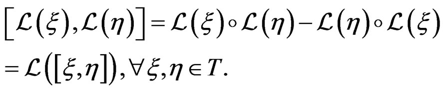
We now recall a few basic geometric concepts that will be constantly used through this paper. First of all, if , we define their bracket
 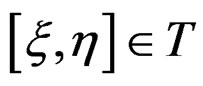 by the local formula
leading to the Jacobi identity
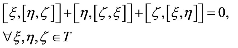
allowing to define a Lie algebra and to the useful formula
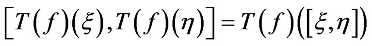
where  is the tangent mapping of a map
 .
.
When  is a multi-index, we may set
for describing  by means of a basis and introduce the exterior derivative
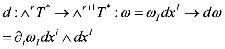
with  in the Poincaré sequence:
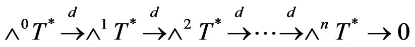 .
.
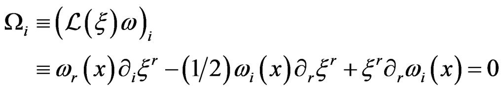
The Lie derivative of an  -form with respect to a vector field
  is the linear first order operator
  linearly depending on
  and uniquely defined by the following three properties:
1)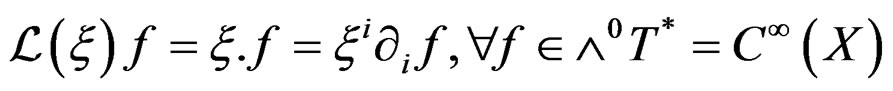 .
.
2)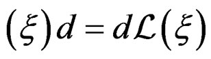 .
.
3) 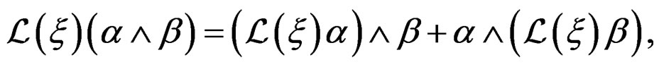
 .
.
It can be proved that

where  is the interior multiplication
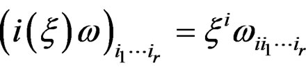
and that
We now turn to group theory and start with two basic definitions:
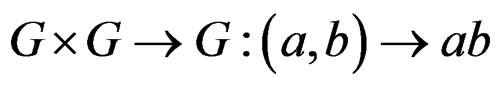
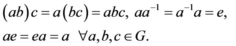
Let  be a Lie group, that is a manifold with local coordinates
  for
for  called parameters, a composition
 an inverse
 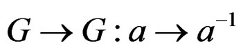 and an identity
  satisfying:
DEFINITION 1.4:  is said to act on
  if there is a map
 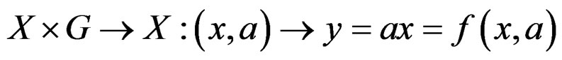 such that
 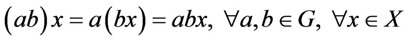 and we shall say that we have a Lie group of transformations of
 . In order to simplify the notations, we shall use global notations even if only local actions are existing. It is well known that the action of
  onto itself allows to introduce a purely algebraic bracket on its Lie algebra
 .
.
DEFINITION 1.5: A Lie pseudogroup of transformations  is a group of transformations solutions of a system of OD or PD equations such that, if
  and
and  are two solutions, called finite transformations, that can be composed, then
and

are also solutions while  is the identity solution denoted by
  and we shall set
 . In all the sequel we shall suppose that
 ![]() is transitive that is
is transitive that is
 .
.
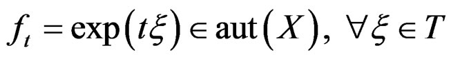
It becomes clear that Lie groups of transformations are particular cases of Lie pseudogroups of transformations as the system defining the finite transformations can be obtained by eliminating the parameters among the equations
when  is large enough. The underlying system may be nonlinear and of high order. Looking for transformations “close” to the identity, that is setting
  when
when  is a small constant parameter and passing to the limit
 , we may linearize the above nonlinear system of finite Lie equations in order to obtain a linear system of infinitesimal Lie equations of the same order for vector fields. Such a system has the property that, if
  are two solutions, then
  is also a solution. Accordingly, the set
  of solutions of this new system satisfies
  and can therefore be considered as the Lie algebra of
![]() .
.
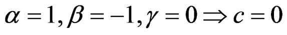
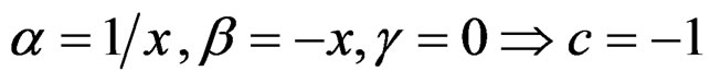
EXAMPLE 1.6: While the affine transformations  are solutions of the second order linear system
 , the projective transformations
are solutions of the third order nonlinear system
 .
.
The sections of the corresponding linearized systems are respectively satisfying  and
and . The generating differential invariant
  of the affine case transforms like
when  while
while  transforms like
 .
.
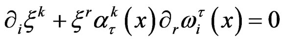
We now sketch the discovery of Vessiot [8,9] still not known today after more than a century for reasons which are not scientific at all. Roughly, a Lie pseudogroup  is made by finite transformations
  solutions of a (possibly nonlinear) system
  while the infinitesimal transformations
  are solutions of the linearized system
as we have
 .
.
When ![]() is transitive, there is a canonical epimorphism
is transitive, there is a canonical epimorphism . Also, as changes of source
 ![]() commute with changes of target
commute with changes of target![]() , they exchange between themselves any generating set of differential invariants
, they exchange between themselves any generating set of differential invariants  as in the previous example.Then one can introduce a natural bundle
  over
over , also called bundle of geomeric objects, by patching changes of coordinates of the form
thus obtained. A section ![]() of
of  is called a geometric object or structure on
  and transforms like
or simply . This is a way to generalize vectors and tensors
  or even connections
 . As a byproduct we have
and we may say that ![]() preserves
preserves![]() . Replacing
. Replacing  by
by , we also obtain
 .
.
Coming back to the infinitesimal point of view and setting
 we may define the ordinary Lie derivative with value in the vector bundle
  by the formula:
and we say that  is a Lie operator because
 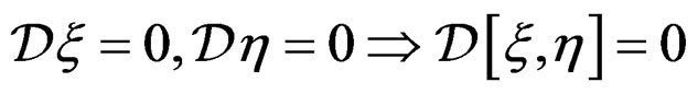 as we already saw.
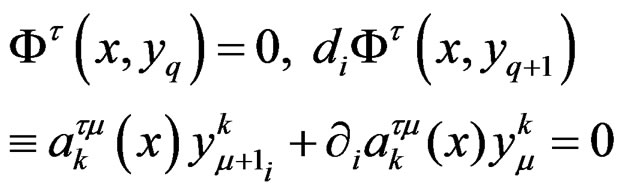
Differentiating  times the equations of
  that only depend on
 , we may obtain the
  - prolongation
 .
.
The problem is then to know under what conditions on ![]() all the equations of order
all the equations of order  are obtained by
  prolongations only,
  or, equivalently,
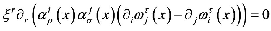
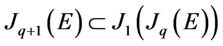
  is formally integrable (FI). The solution, found by Vessiot, has been to exhibit another natural vector bundle
  with local coordinates
  over
over  with local coordinates
  and to prove that an equivariant section
  only depends on a finite number of constants called structure constants. The integrability conditions (IC) of
 , called Vessiot structure equations, are of the form
  and are invariant under any change of source.
We provide in a self-contained way and parallel manners the following five striking examples which are among the best nontrivial ones we know and invite the reader to imagine at this stage any possible link that could exist between them (A few specific definitions will be given later on).
EXAMPLE 1.7: Coming back to the last example, we show that Vessiot structure equations may even exist when . For this, if
  is the geometric object of the affine group
  and
and  is a
is a  -form, we consider the object
  and get at once the two second order Medolaghi equations:
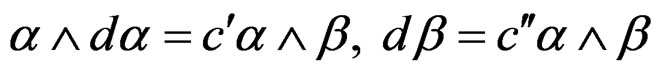
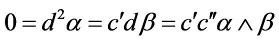
Differentiating the first equation and substituting the second, we get the zero order equation:
and the Vessiot structure equation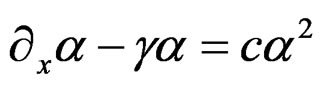 . Alternatively, setting
 we get
 .
.
With
we get the translation subgroup 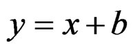 while, with
we get the dilatation subgroup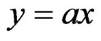 . Similarly, if
 ![]() is the geometric object of the projective group and we consider the new geometric object
is the geometric object of the projective group and we consider the new geometric object , we get the only Vessiot structure equation
without any structure constant.
EXAMPLE 1.8: (Principal homogeneous structure) When ![]() is the Lie group of transformations made by the constant translations
is the Lie group of transformations made by the constant translations  for
for  of a manifold
  with
with , the characteristic object invariant by
 ![]() is a family
is a family
of ![]()
 -forms with
  in such a way that

where  denotes the pseudogroup of local diffeomorphisms of
 ,
,  denotes the derivatives of
 up to order
  and
and  acts in the usual way on covariant tensors. For any vector field
  the tangent bundle to
 , introducing the standard Lie derivative
  of forms with respect to
 , we may consider the
  first order Medolaghi equations:
 .
.
The particular situation is found with the special choice  that leads to the involutive system
 . Introducing the inverse matrix
 , the above equations amount to the bracket relations
  and, using crossed derivatives on the solved form
 we obtain the
  zero order equations:
 .
.
The integrability conditions (IC), that is the conditions under which these equations do not bring new equations, are thus the  Vessiot structure equations:
with 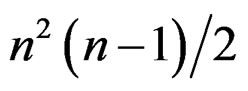 structure constants
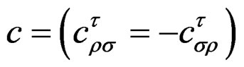 .
.
When , these equations can be identified with the Maurer-Cartan equations (MC) existing in the theory of Lie groups, on the condition to change the sign of the structure constants involved because we have
 .
.
Writing these equations in the form of the exterior system 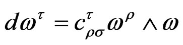 and closing this system by applying once more the exterior derivative
![]() , we obtain the quadratic IC:
, we obtain the quadratic IC:
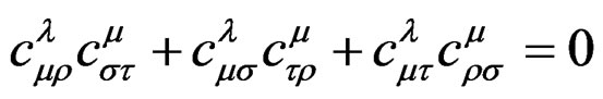
also called Jacobi relations .
.
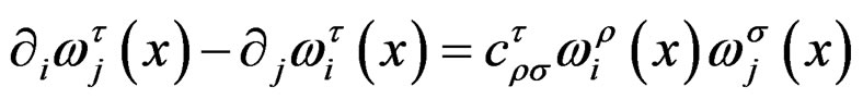
EXAMPLE 1.9: (Riemann structure) If
is a metric on a manifold  with
with  such that
 , the Lie pseudogroup of transformations preserving
 ![]() is
is
and is a Lie group with a maximum number of  parameters. A special metric could be the Euclidean metric when
  as in elasticity theory or the Minkowski metric when
 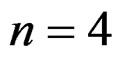 as in special relativity [10]. The first order Medolaghi equations:
are also called classical Killing equations for historical reasons. The main problem is that this system is not involutive unless we prolong it to order two by differentiating once the equations. For such a purpose, introducing 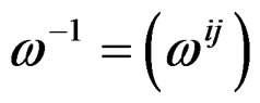 as usual, we may define the Christoffel symbols:
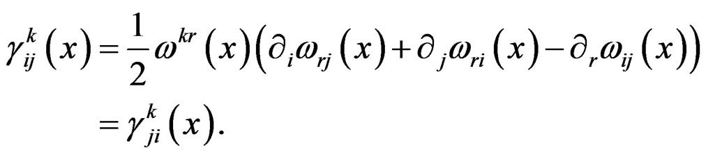
This is a new geometric object of order 2 providing the Levi-Civita isomorphism  of affine bundles and allowing to obtain the second order Medolaghi equations:
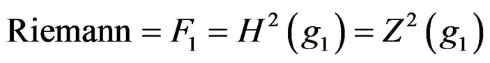
Surprisingly, the following expression called Riemann tensor:
is still a first order geometric object and even a  -tensor with
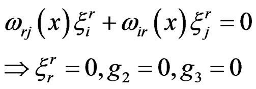
 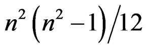 independent components satisfying the purely algebraic relations:
 .
.
Accordingly, the IC must express that the new first order equations 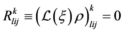 are only linear combinations of the previous ones and we get the Vessiot structure equations:
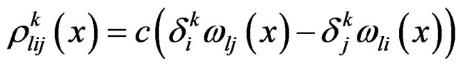
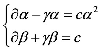
with the only structure constant ![]() describing the constant Riemannian curvature condition of Eisenhart [11,12]. One can proceed similarly for the conformal Killing system
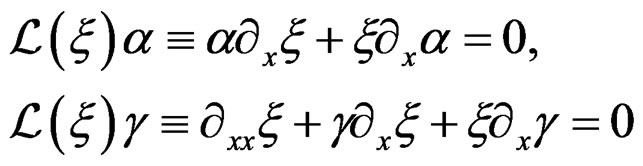
describing the constant Riemannian curvature condition of Eisenhart [11,12]. One can proceed similarly for the conformal Killing system 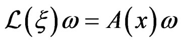 and obtain that the Weyl tensor must vanish, without any structure constant [12].
EXAMPLE 1.10: (Contact structure) We only treat the case  as the case
  needs much more work [6]. Let us consider the so-called contact
  -form
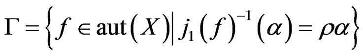
-form 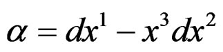 and consider the Lie pseudogroup
  of (local) transformations preserving
 ![]() up to a function factor, that is
up to a function factor, that is
where again  is a symbolic way for writing out the derivatives of
  up to order
  and
and ![]() transforms like a
transforms like a  -covariant tensor. It may be tempting to look for a kind of “object” the invariance of which should characterize
![]() . Introducing the exterior derivative
. Introducing the exterior derivative  as a
as a  -form, we obtain the volume
  -form
-form . As it is well known that the exterior derivative commutes with any diffeomorphism, we obtain sucessively:
As the volume  -form
-form  transforms through a division by the Jacobian determinant
of the transformation  with inverse
 the desired object is thus no longer a 1-form but a 1- form density
  transforming like a 1- form but up to a division by the square root of the Jacobian determinant. It follows that the infinitesimal contact transformations are vector fields
  the tangent bundle of
 , satisfying the 3 so-called first order Medolaghi equations:
 .
.
When , we obtain the special involutive system:
with 2 equations of class 3 and 1 equation of class 2 (see later on for a precise definition) and thus only 1 compatibility conditions (CC) for the second members.
For an arbitrary![]() , we may ask about the differential conditions on
, we may ask about the differential conditions on ![]() such that all the equations of order
such that all the equations of order  are only obtained by differentiating
  times the first order equations, exactly like in the special situation just considered where the system is involutive. We notice that, in a symbolic way,
  is now a scalar
  providing the zero order equation
  and the condition is
 . The integrability condition (IC) is the Vessiot structure equation:
involving the only structure constant![]() .
.
For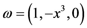 , we get
 . If we choose
  leading to
 , we may define
with infinitesimal transformations satisfying the involutive system:
with again 2 equations of class 3 and 1 equation of class 2.
EXAMPLE 1.11: (Unimodular contact structure) With similar notations, let us again set
but let us now consider the new Lie pseudogroup of transformations preserving ![]() and thus
and thus  too, that is preserving the mixed object
made up by a  -form
-form ![]() and a
and a  -form
-form  with
with
 and
and .
.
Then ![]() is a Lie subpseudogroup of the one just considered in the previous example and the corresponding infinitesimal transformations now satisfy the involutive system:
is a Lie subpseudogroup of the one just considered in the previous example and the corresponding infinitesimal transformations now satisfy the involutive system:

with 3 equations of class 3, 2 equations of class 2 and  equation of class 1 if we exchange
  with
with , a result leading now to 4 CC.
More generally, when  where
where ![]() is a 1- form and
is a 1- form and  is a
is a  -form satifying
 , we may study the same problem as before for the general system
 .
.
We let the reader provide the details of the tedious computation involved as it is at this point that computer algebra may be used [13]. The result, not evident at first sight, is that the 2-form  must be proportional to the 2-form
 , that is
  and thus
 .
.
As , we must have
  and thus
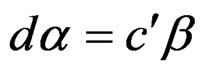 . Similarly, we get
 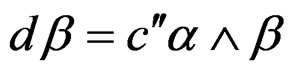 and obtain finally the
  Vessiot structure equations
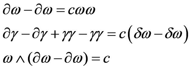
involving 2 structure constants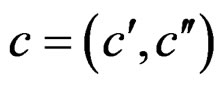 . Contrary to the previous situation (but like in the Riemann case!) we notice that we have now 2 structure equations not containing any constant (called first kind by Vessiot) and 2 structure equations with the same number of different constants (called second kind by Vessiot), namely
 .
.
Finally, closing this system by taking once more the exterior derivative, we get
and thus the unexpected purely algebraic Jacobi condition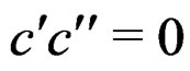 . For the special choice
we get , for the second special choice
we get  and for the third special choice
we get .
.
FIRST FUNDAMENTAL RESULT: Comparing the various Vessiot structure equations containing structure constants that we have just presented and that we recall below in a symbolic way, we notice that these structure constants are absolutely on equal footing though they have in general nothing to do with any Lie algebra.
 .
.
Accordingly, the fact that the ones appearing in the MC equations are related to a Lie algebra is a coincidence and the Cartan structure equations have nothing to do with the Vessiot structure equations. Also, as their factors are either constant, linear or quadratic, any identification of the quadratic terms appearing in the Riemann tensor with the quadratic terms appearing in the MC equations is definitively not correct [7]. We also understand why the torsion is automatically combined with curvature in the Cartan structure equations but totally absent from the Vessiot structure equations, even though the underlying group (translations + rotations) is the same.
HISTORICAL REMARK 1.12: Despite the prophetic comments of the italian mathematician Ugo Amaldi in 1909 [12], it has been a pity that Cartan deliberately ignored the work of Vessiot at the beginning of the last century and that the things did not improve afterwards in the eighties with Spencer and coworkers (Compare MR 720863 (85 m: 12004) and MR 954613 (90e: 58166)).
3. Second Part: The Janet and Spencer Sequences
Let  be a multi-index with length
class  if
if
and
 .
.
We set
with  when
when . If
. If  is a vector bundle over
  with local coordinates
  and
and  is the
  -jet bundle of
  with local coordinates
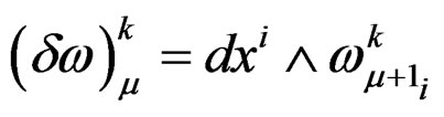
 the Spencer operator just allows to distinguish a section
  from a section
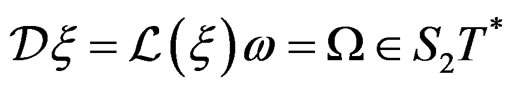
  by introducing a kind of “difference” through the operator

with local components
and more generally
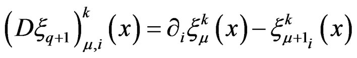 .
.
Minus the restriction of  to the kernel
 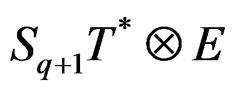 of the canonical projection
can be extended to the Spencer map
defined by
 .
.
The kernel of  is made by sections such that
 .
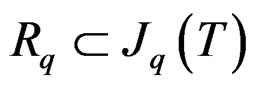
.
Finally, if 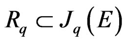 is a system of order
  on
on  locally defined by linear equations
 the
the  -prolongation
is locally defined when  by the linear equations
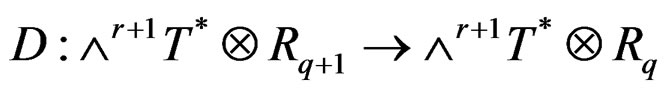
and has symbol
locally defined by
if one looks at the top order terms. If  is over
 , differentiating the identity
with respect to  and substracting the identity
![]() we obtain the identity
we obtain the identity
and thus the restriction . This first order operator induces, up to sign, the purely algebraic monomorphism
 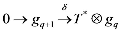 on the symbol level
[8,14]. The Spencer operator has never been used in GR though an accelerometer in a rocket merely measures one of the components of the Spencer operator involving second order jets.
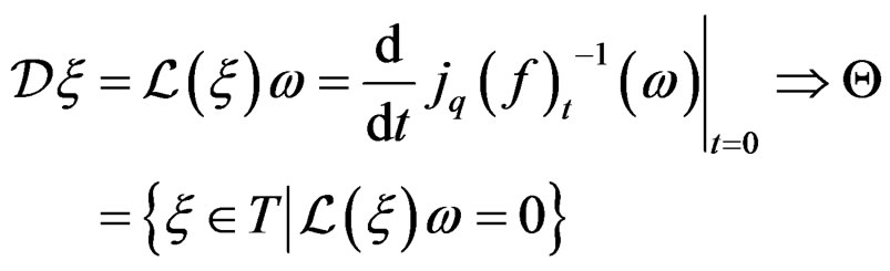
DEFINITION 2.1:  is said to be formally integrable (FI) when the restriction
is an epimorphism . In that case, the Spencer form
  is a canonical equivalent formally integrable first order system on
  with no zero order equations.
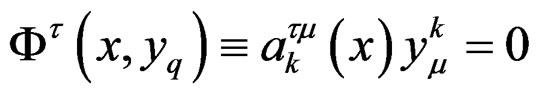
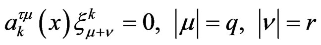
DEFINITION 2.2:  is said to be involutive when it is formally integrable and the symbol
  is involutive, that is all the sequences
are exact . Equivalently, using a linear change of local coordinates if necessary, we may successively solve the maximum number
  of equations with respect to the leading or principal jet coordinates of strict order
  and class
 . Then
  is involutive if
  is obtained by only prolonging the
  equations of class
  with respect to
  for
for . In that case, such a prolongation procedure allows to compute in a unique way the principal jets from the parametric other ones and may also be applied to nonlinear systems as well [8,15].
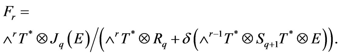
When  is involutive, the linear differential operator
of order  with space of solutions
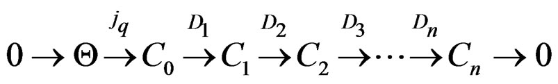
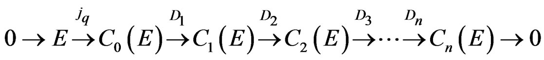
  is said to be involutive and one has the canonical linear Janet sequence [8]:
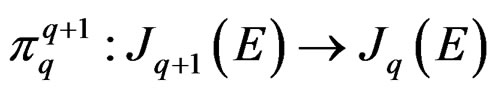
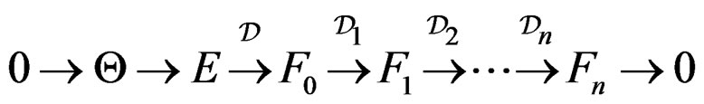
with Janet bundles
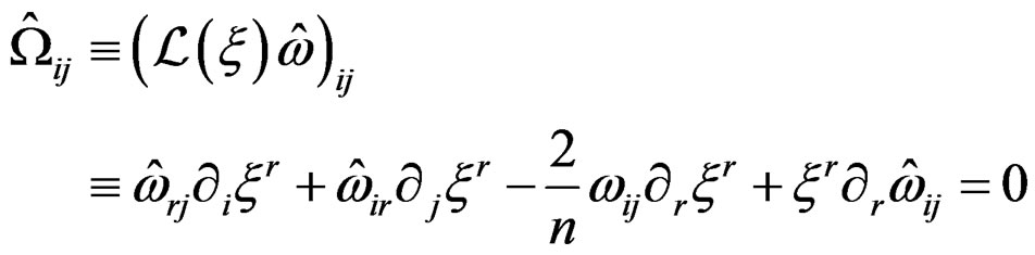
Each operator 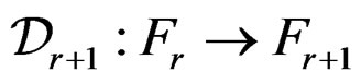 is first order involutive as it is induced by
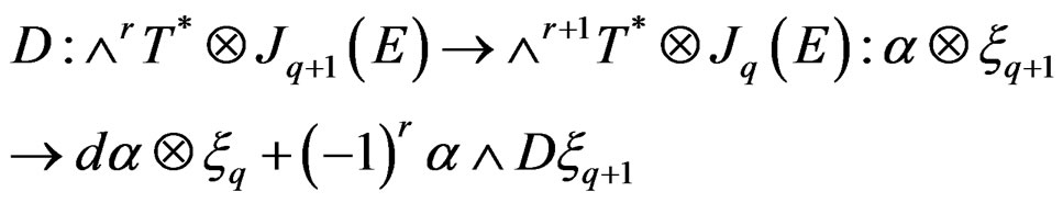
and generates the compatibility conditions (CC) of the preceding one. As the Janet sequence can be cut at any place, the numbering of the Janet bundles has nothing to do with that of the Poincaré sequence, contrary to what many people believe in GR.
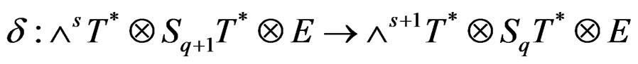
Similarly, we have the involutive first Spencer operator
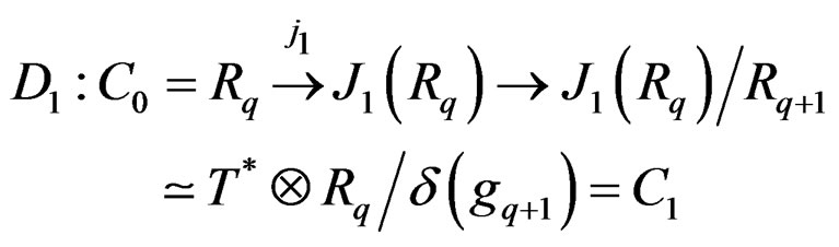
of order one induced by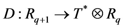 . Introducing the Spencer bundles
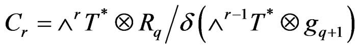 the first order involutive
  Spencer operator
 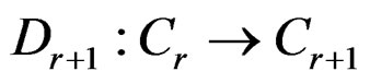 is induced by
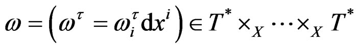
and we obtain the canonical linear Spencer sequence [8,14]:
as the Janet sequence for the first order involutive system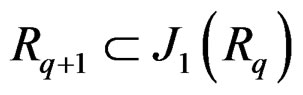 . Introducing the other Spencer bundles

with , the linear Spencer sequence is induced by the linear hybrid sequence:
which is at the same time the Janet sequence for  and the Spencer sequence for
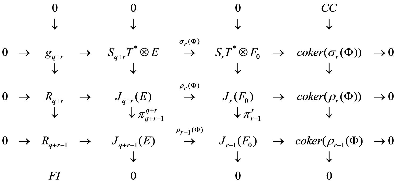
[8,14]. Such a sequence projects onto the Janet sequence and we have the following commutative diagram with exact columns:
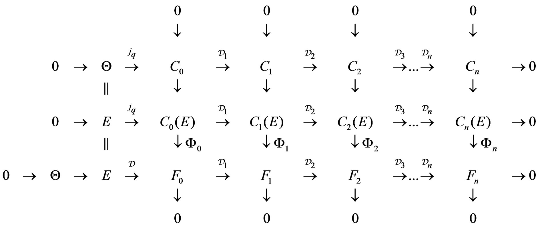
In this diagram, only depending on the linear differential operator , the epimorhisms
 for
for 
are induced by the canonical projection

if we start with the knowledge of  or from the knowledge of an epimorphism
if we set . In the theory of Lie equations considered,
  ,
,  is a transitive involutive system of infinitesimal Lie equations of order
  and the corresponding operator
  is a Lie operator. As an exercise, we invite the reader to draw this diagram in the affine and projective 1-dimensional cases.
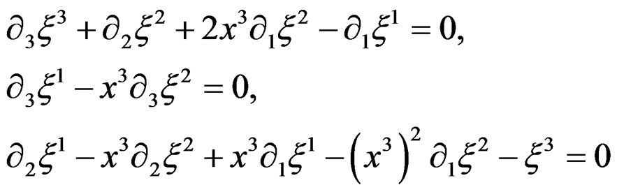
EXAMPLE 2.3: If we restrict our study to the group of isometries of the euclidean metric ![]() in dimension
in dimension , exhibiting the Janet and the Spencer sequences is not easy at all, even when
 , because the corresponding Killing operator
 involving the Lie derivative
  and providing twice the so-called infinitesimal deformation tensor
 ![]() of continuum mechanics, is not involutive. In order to overcome this problem, one must differentiate once by considering also the Christoffel symbols
of continuum mechanics, is not involutive. In order to overcome this problem, one must differentiate once by considering also the Christoffel symbols  and add the operator
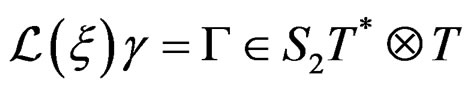 .
.
Now, one can prove that the Spencer sequence for Lie groups of transformations is locally isomorphic to the tensor product of the Poincaré sequence by the Lie algebra of the underlying Lie group [7,8]. Hence, if two Lie groups  act on
 , it follows from the definition of the Janet and Spencer bundles that the Spencer sequence for
  is embedded into the Spencer sequence for
  while the Janet sequence for
  projects onto the Janet sequence for
  but the common differences are isomorphic to
 . This rather philosophical comment, namely to replace the Janet sequence by the Spencer sequence, must be considered as the crucial key for understanding the work of the brothers E. and F. Cosserat in 1909 [7,17-19] or H. Weyl in 1918 [7,16], the best picture being that of Janet and Spencer playing at see-saw. Indeed, when
 , one has 3 parameters (2 translations + 1 rotation) and the following commutative diagram which only depends on the left commutative square:
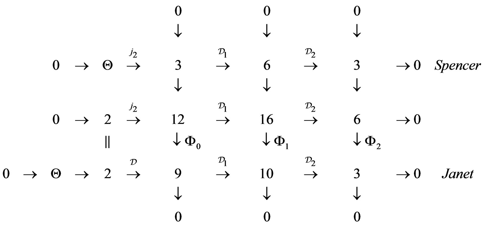
In this diagram, there is no way to compare  (curvature alone as in Vessiot) with
  (curvature + torsion as in Cartan).
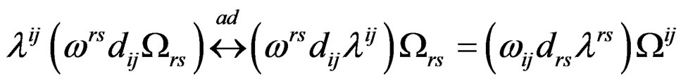
For proving that the adjoint of  provides the Cosserat equations which can be parametrized by the adjoint of
 , we may lower the upper indices by means of the constant euclidean metric and look for the factors of
  and
and  in the integration by parts of the sum:
in order to obtain:
Finally, we get the nontrivial first order parametrization
by means of the three arbitrary functions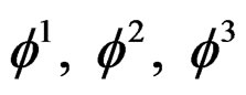 , in a coherent way with the Airy second order parametrization obtained if we set
when 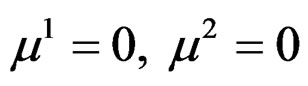 as we shall see in the third part.
The link between the FI of  and the CC of
  is expressed by the following diagram that may be used inductively:
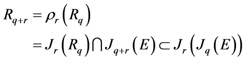
The “snake theorem” [8,20] then provides the long exact connecting sequence:
 .
.
If we apply such a diagram to first order Lie equations with no zero or first order CC, we have 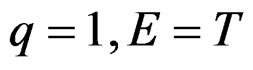 and we may apply the Spencer
 ![]() -map to the top row obtained with r = 2 in order to get the commutative diagram:
-map to the top row obtained with r = 2 in order to get the commutative diagram:
with exact rows and exact columns but the first that may not be exact at . We shall denote by
  the coboundary as the image of the central
![]() , by
, by  the cocycle as the kernel of the lower
 ![]() and by
and by  the Spencer
 ![]() -cohomology at
-cohomology at  as the quotient.
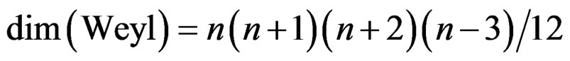
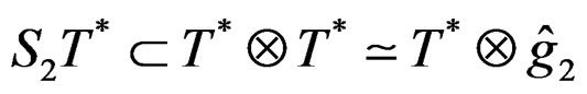
In the classical Killing system, 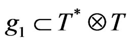 is defined by
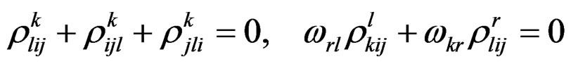
Applying the previous diagram, we discover that the Riemann tensor is a section of the bundle
with
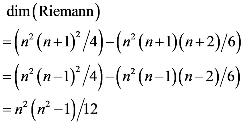
by using the top row or the left column. Though we discover the two properties of the Riemann tensor through the chase involved, we have no indices and cannot therefore exhibit the Ricci tensor of GR by means of the usual contraction or trace.
Let us proceed the same way with the conformal Killing system
obtained by introducing
or, equivalently, by eliminating  in
in
 .
.
Now  is defined by
but we have  with
with 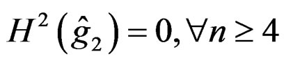 and the Weyl tensor is a section of the bundle
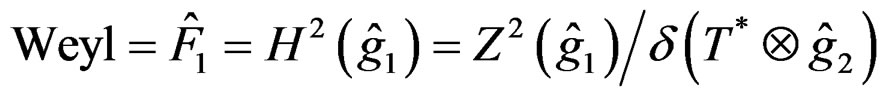
with
 .
.
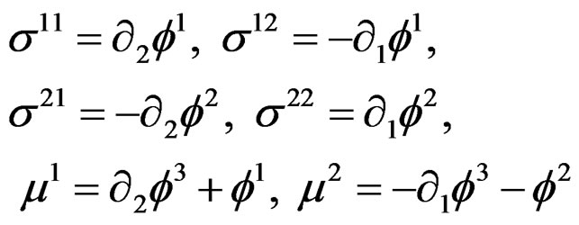
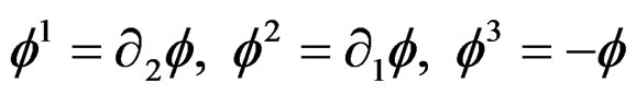
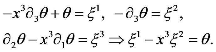
Similarly, we have no indices and cannot therefore exhibit the Ricci tensor. However, when , among the components of the Spencer operator we have
and thus
 .
.
Such a result allows to recover the electromagnetic field in the image of the Spencer operator  and Maxwell equations by duality along the way proposed by Weyl in [16] but the use of the Spencer operator provides the only possibility to exhibit a link with Cosserat equations.
Comparing the classical and conformal Killing systems by using the inclusions
 we finally obtain the following commutative and exact diagram where a diagonal chase allows to identify
  with
with
and to split the right column [7,12,20]:
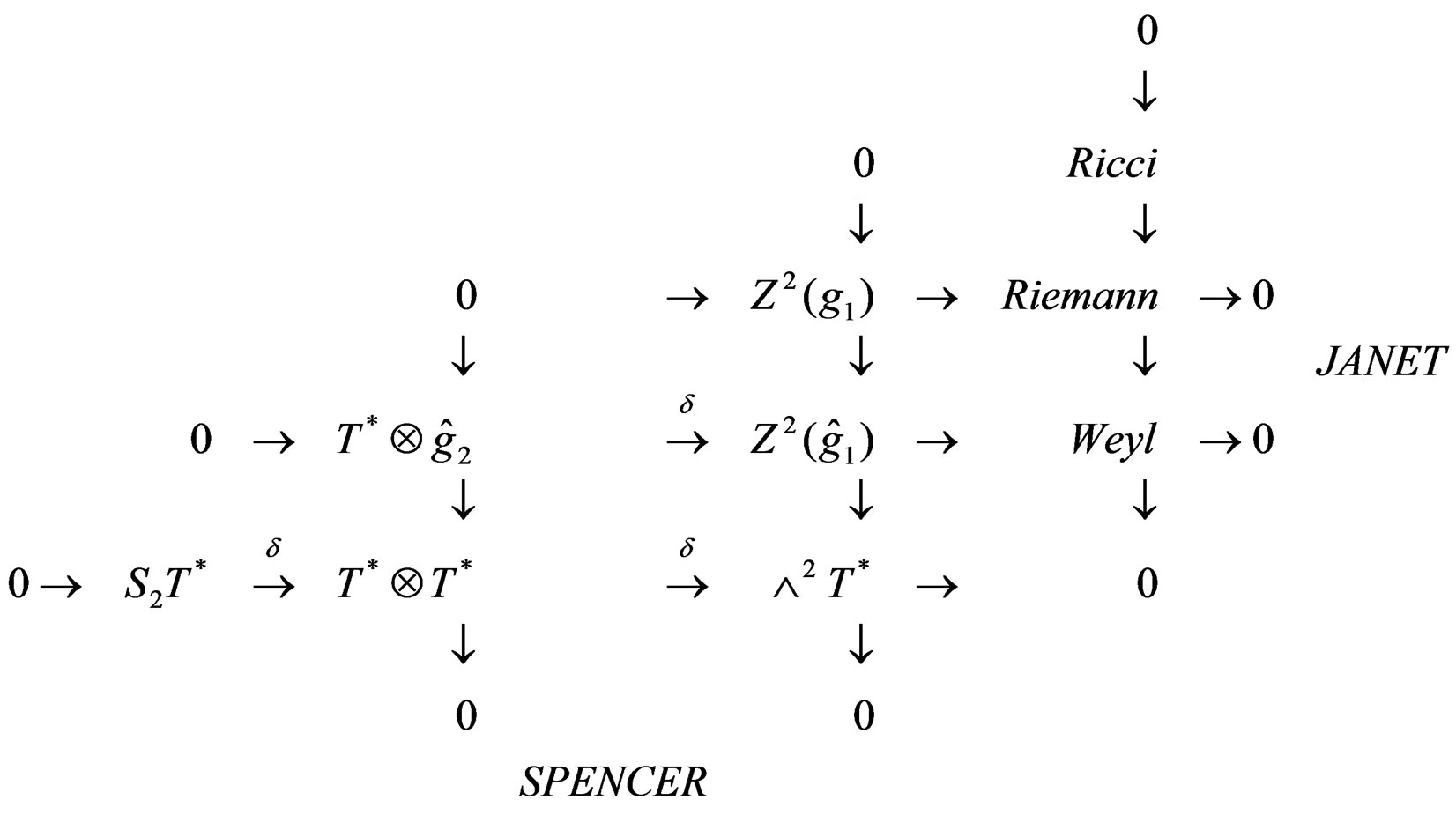
SECOND FUNDAMENTAL RESULT: The Ricci tensor only depends on the “difference” existing between the clasical Killing system and the conformal Killing system, namely the ![]() second order jets (elations once more). The Ricci tensor, thus obtained without contracting the indices as usual, may be embedded in the image of the Spencer operator made by 1-forms with value in 1-forms that we have already exhibited for describing EM. It follows that the foundations of both EM and GR are not coherent with jet theory and must therefore be revisited within this new framework.
second order jets (elations once more). The Ricci tensor, thus obtained without contracting the indices as usual, may be embedded in the image of the Spencer operator made by 1-forms with value in 1-forms that we have already exhibited for describing EM. It follows that the foundations of both EM and GR are not coherent with jet theory and must therefore be revisited within this new framework.
4. Third Part: Algebraic Analysis
EXAMPLE 3.1: Let a rigid bar be able to slide along an horizontal axis with reference position ![]() and attach two pendula, one at each end, with lengths
and attach two pendula, one at each end, with lengths  and
and![]() , having small angles
, having small angles  and
and  with respect to the vertical. If we project Newton law with gravity
 ![]() on the perpendicular to each pendulum in order to eliminate the tension of the threads and denote the time derivative with a dot, we get the two equations:
on the perpendicular to each pendulum in order to eliminate the tension of the threads and denote the time derivative with a dot, we get the two equations:
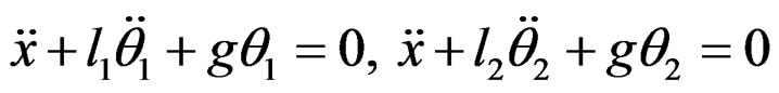
As an experimental fact, starting from an arbitrary movement of the pendula, we can stop them by moving the bar if and only if 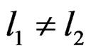 and we say that the system is controllable.
More generally, we can bring the OD equations describing the behaviour of a mechanical or electrical system to the Kalman form 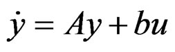 with input
 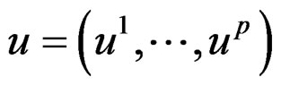 and output
 . We say that the system is controllable if, for any given
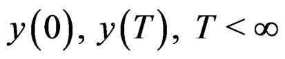 one can find
 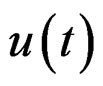 such that a coherent trajectory
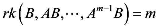
  may be found. In 1963 [21], R. E. Kalman discovered that the system is controllable if and only if
 .
.
Surprisingly, such a functional definition admits a formal test which is only valid for Kalman type systems with constant coefficients and is thus far from being intrinsic. In the PD case, the Spencer form will replace the Kalman form.
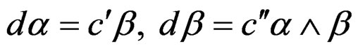
EXAMPLE 3.2:
can always be achieved and the system is thus controllable in the sense of the definition but  is not controllable in the sense of the test.
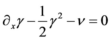
EXAMPLE 3.3:
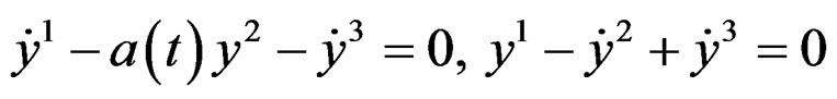 .
.
Any way to bring this system to Kalman form provides the controllability condition  if
if  but nothing can be said if
 . Also, getting
  from the second equation and substituting in the first, we get the second order OD equation
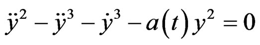
for which nothing can be said at first sight.
PROBLEM 1: Is a SYSTEM of OD or PD equations “controllable” (answer must be YES or NO) and how can we define controllability?
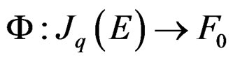
Now, if a differential operator  is given, a direct problem is to find (generating) compatibility conditions (CC) as an operator
  such that
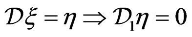 .
.
Conversely, the inverse problem will be to find 
such that  generates the CC of
  and we shall say that
  is parametrized by
 . Of course, solving the direct problem (Janet, Spencer) is necessary for solving the inverse problem.
EXAMPLE 3.4: When , the Cauchy equations for the stress in continuum mechanics are
with .
.
Their parametrization
has been discovered by Airy in 1862 and  is called the Airy function. When
 , Maxwell and Morera discovered a similar parametrization with 3 potentials (exercise).
EXAMPLE 3.5: When , the Maxwell equations
  where
where  is the EM field are parametrized by
  where
where  is the 4-potential. The second set of Maxwell equations can also be parametrized by the so-called pseudopotential which is a pseudovector density (exercise).
EXAMPLE 3.5: If ,
, ![]() is the Minkowski metric and
is the Minkowski metric and 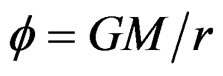 is the gravitational potential, then
 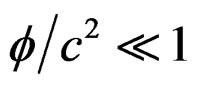 and a perturbation
  of
of ![]() may satisfy in vacuum the 10 second order Einstein equations for the 10
may satisfy in vacuum the 10 second order Einstein equations for the 10 :
:
The parametrizing challenge has been proposed in 1970 by J. Wheeler for 1000 $ and solved negatively in 1995 by the author who only received 1 $.
PROBLEM 2: Is an OPERATOR parametrizable (answer must be YES or NO) and how can we find a parametrization?
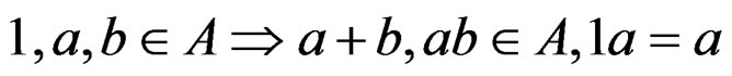
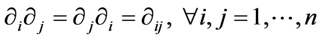
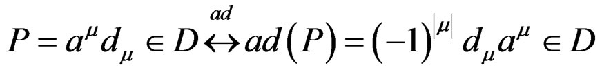
Let  be a unitary ring, that is
and even an integral domain, that is
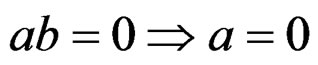 or
or .
.
We say that  is a left module over
  if
if

and we denote by  the set of morphisms
 such that
 .
.
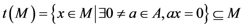
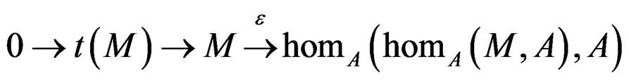
DEFINITION 3.6: We define the torsion submodule
 .
.
There is a sequence
where the morphism ![]() is defined by
is defined by

because we have at once
 .
.
PROBLEM 3: Is a MODULE  torsion-free, that is
  (answer must be YES or NO) and how can we test such a property?
In the remaining of this paper we shall prove that the three problems are indeed identical and that only the solution of the third will provide the solution of the two others [1,22-24].
Let 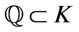 be a differential field, that is a field
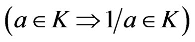
with ![]() commuting derivations
commuting derivations 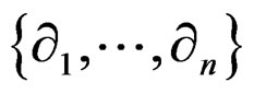 with
with
such that
and
 .
.
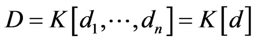
Using an implicit summation on multiindices, we may introduce the (noncommutative) ring of differential operators
with elements  such that
  and
and 
 . Now, if we introduce differential indeterminates
 , we may extend
 ![]() to
to
for . Therefore, setting
 we obtain by residue the differential module or
  - module
 . Introducing the two free differential modules
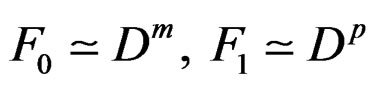 , we obtain equivalently the free presentation
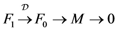 . More generally, introducing the successive CC as in the preceding section, we may finally obtain the free resolution of
 , namely the exact sequence
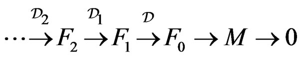 .
.
The “trick” is to let  act on the left on column vectors in the operator case and on the right on row vectors in the module case. Homological algebra has been created for finding intrinsic properties of modules not depending on their presentation or even on their resolution.
EXAMPLE 3.7: In order to understand that different presentations may nevertheless provide isomorphic modules, let us consider the linear inhomogeneous system 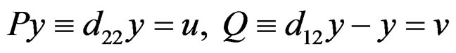 with
with . Differentiating twice, we get
  and the two fourth order CC:
However, as , we also get the CC
 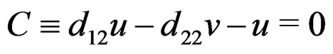 and the two resolutions:
where we can identify the two differential modules involved on the right with  because:
We now exhibit another approach by defining the formal adjoint of an operartor  and an operator matrix
 :
:
DEFINITION 3.8:
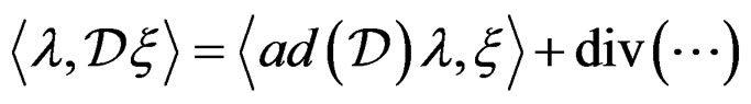
from integration by part, where ![]() is a row vector of test functions and
is a row vector of test functions and  the usual contraction.
PROPOSITION 3.9: If we have an operator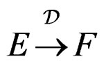 , we obtain by duality an operator
where  is obtained from
  by inverting the transition matrix and EM provides a fine example of such a procedure [10].
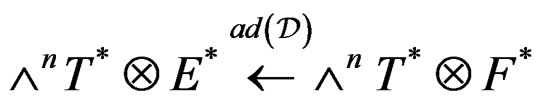
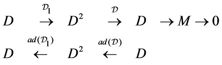
Now, with operational notations, let us consider the two differential sequences:
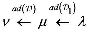
where  generates all the CC of
 . Then
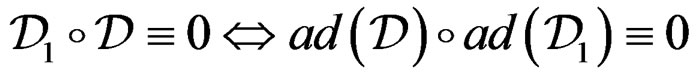
but  may not generate all the CC of
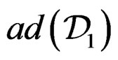 .
.
EXAMPLE 3.10: With 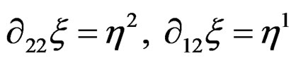 for
for , we get
 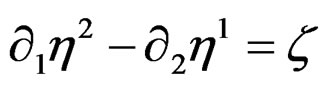 for
for . Then
  is defined by
 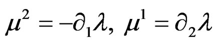 while
while  is defined by
  but the CC of
  are generated by
 . Passing to the module framework, we obtain the sequences:
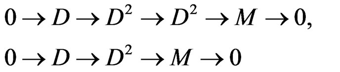
THEOREM 3.11: The cohomology 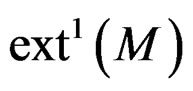 at
at  of the lower sequence does not depend on the resolution of
  and is a torsion module called the first extension module of
 .
.
Exactly like we defined the differential module  from
from , let us define the differential module
  from
from . The proof of the next theorem is quite tricky and out of the scope of this paper [1,22-24]:
MAIN THEOREM 3.12: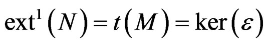 .
.
FORMAL TEST 3.13: The double duality test needed in order to check whether 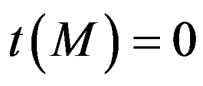 or not and to find out a parametrization if
  has 5 steps which are drawn in the following diagram where
 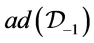 generates the CC of
 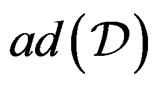 and
and  generates the CC of
 :
:
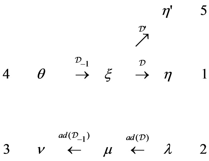
THEOREM 3.14:  parametrized by
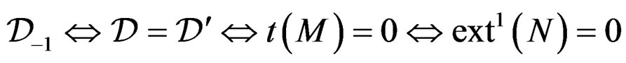 .
.
COROLLARY 3.15: If  and
and  is surjective, then
  if and only if
  is injective [24,25].
EXAMPLE 3.16: (Kalman test revisited) If we multiply the Kalman system 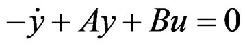 on the left by a test row vector
![]() , we obtain:
, we obtain:
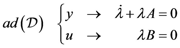
Differentiating the zero order equations and using the first order ones, we get 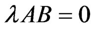 and so on. Using the Cayley-Hamilton theorem, we stop at
 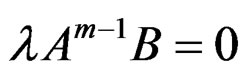 and find back exactly the Kalman test but in a completely different intrinsic framework.
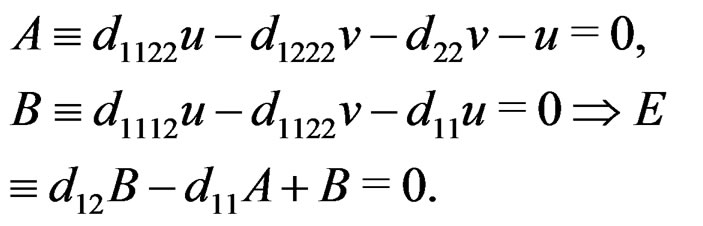
EXAMPLE 3.17: (Double pendulum revisited) Using two test functions  and
and , we get:
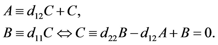
and obtain at once the zero order equation
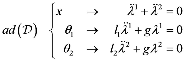
 .
.
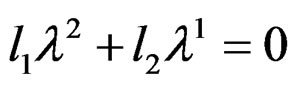
Differentiating twice and substituting, we also get
 and
and  is injective if and only if
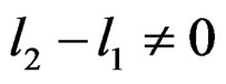 .
.
EXAMPLE 3.18: (Airy parametrization revisited) When , we may study the infinitesimal deformation
  by means of the Killing operator
 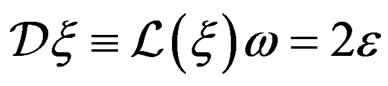 when
when ![]() is the euclidean metric. Then
is the euclidean metric. Then  provides (up to sign and factor
 ) the Cauchy equations
 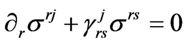 for the stress tensor density [12,16,26]. The following diagram describes the Poincaré scheme:
 .
.
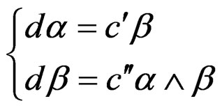
Accordingly, the second order Airy parametrization is nothing else than the adjoint of the only Riemann CC involved, namely 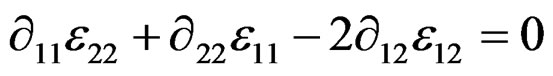 which is the linearization of the Riemann tensor of Example 1.9.
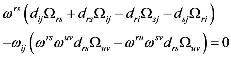
EXAMPLE 3.19: (Einstein equations revisited) Contrary to the Ricci operator, the Einstein operator is selfadjoint because it comes from a variational procedure, the sixth terms being exchanged between themselves under . For example, we have:
and the adjoint of the first operator is the sixth. Accordingly, one has the following diagram where :
:
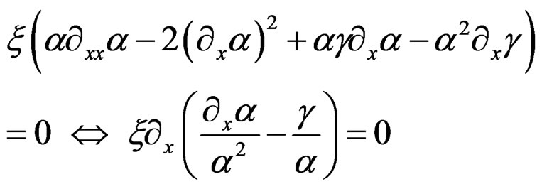
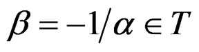
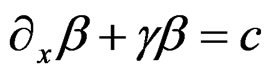
THIRD FUNDAMENTAL RESULT: Comparing this diagram to the previous one proves that Einstein equations are not coherent with Janet and Spencer sequences as conformal geometry has not been introduced in this last part.
EXERCISE 3.20: Prove that

is controllable if and only if 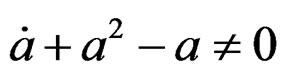 (Riccati) and find a parametrization.
EXERCISE 3.21: Prove that the infinitesimal contact transformations of Example 1.10 admit the injective parametrization
5. Conclusion
The mathematical foundations of General Relativity leading to Einstein equations are always presented in textbooks or papers without any reference to conformal geometry. However, comparing the classical Killing equations to the conformal Killing equations while constructing corresponding differential sequences, the Ricci tensor appears as the kernel of the canonical projection of the Riemann tensor onto the Weyl tensor. After obtaining such a result in a purely intrinsic way, that is without using indices, we have been able to introduce “diagram chasing” in order to relate for the first time electromagnetism and gravitation to the Spencer ![]() -cohomology of the classical and conformal Killing symbols. Accordingly, the mathematical foundations of general relativity are not coherent with jet theory and must therefore be revisited within this new framework along the lines we have sketched. Finally, the fact that Einstein equations cannot be parametrized, contrary to most other equations of physics or engineering, also brings a deep structural question on these equations that will have to be solved in the future by means of algebraic analysis.
-cohomology of the classical and conformal Killing symbols. Accordingly, the mathematical foundations of general relativity are not coherent with jet theory and must therefore be revisited within this new framework along the lines we have sketched. Finally, the fact that Einstein equations cannot be parametrized, contrary to most other equations of physics or engineering, also brings a deep structural question on these equations that will have to be solved in the future by means of algebraic analysis.
REFERENCES
- J.-F. Pommaret, “Partial Differential Control Theory,” Kluwer, Dordrecht, 2001. doi:10.1007/978-94-010-0854-9
- E. Cartan, Annales Scientifiques de l’École Normale Supérieure, Vol. 21, 1904, pp. 153-206.
- E. Cartan, Annales Scientifiques de l’École Normale Supérieure, Vol. 40, 1923, pp. 325-412.
- H. Goldschmidt, Journal of Differential Geometry, Vol. 6, 1972, pp. 357-373,
- A. Kumpera and D. C. Spencer, “Lie Equations,” Annals of Mathematics Studies 73, Princeton University Press, Princeton, 1972.
- J.-F. Pommaret, “Differential Galois Theory,” Gordon and Breach, New York, 1983.
- J.-F. Pommaret, “Spencer Operator and Applications: From Continuum Mechanics to Mathematical Physics,” In: Y. Gan, Ed., Continuum Mechanics-Progress in Fundamentals and Engineering Applications, InTech, 2012. http://www.intechopen.com/books/continuum-mechanics-progress-in-fundamentals-and-engineering-applications/spencer-operator-and-applications-from-continuum-mechanics-to-mathematical-physics
- J.-F. Pommaret, “Partial Differential Equations and Group Theory,” Kluwer, 1994. doi:10.1007/978-94-017-2539-2
- E. Vessiot, Annales scientifiques de l’École Normale Supérieure, Vol. 20, 1903, pp. 411-451.
- V. Ougarov, “Théorie de la Relativité Restreinte,” MIR, Moscow, 1969.
- L. P. Eisenhart, “Riemannian Geometry,” Princeton University Press, Princeton, 1926.
- J.-F. Pommaret, “Lie Pseudogroups and Mechanics,” Gordon and Breach, New York, 1988.
- A. Lorenz, “Jet Groupoids, Natural Bundles and the Vessiot Equivalence Method,” Acta Applicandae Mathematicae, Vol. 1, 2008, pp. 205-213. doi:10.1007/s10440-008-9193-7
- D. C. Spencer, Bulletin of the American Mathematical Society, Vol. 75, 1965, pp. 1-114.
- M. Janet, Journal de Mathématiques Pures et Appliquées, Vol. 8, 1920, pp. 65-151.
- H. Weyl, “Space, Time, Matter,” Berlin, 1918.
- E. Cosserat and F. Cosserat, “Théorie des Corps Déformables,” Hermann, Paris, 1909.
- J.-F. Pommaret, Acta Mechanica, Vol. 149, 2001, pp. 23-39. doi:10.1007/BF01261661
- J.-F. Pommaret, Acta Mechanica, Vol. 215, 2010, pp. 43- 55. doi:10.1007/s00707-010-0292-y
- J. J. Rotman, “An Introduction to Homological Algebra,” Academic Press, Cambridge, 1979.
- R. E. Kalman, Y. C. Yo and K. S. Narenda, Journal of Differential Equations, Vol. 1, 1963, pp. 189-213.
- M. Kashiwara, Mémoires de la Société Mathématique de France, Vol. 63, 1995, pp. 1-72.
- V. P. Palamodov, “Linear Differential Operators with Constant Coefficients,” Grundlehren der Mathematischen Wissenschaften 168, Springer, 1970. doi:10.1007/978-3-642-46219-1
- J.-F. Pommaret, “Algebraic Analysis of Control Systems Defined by Partial Differential Equations,” Advanced Topics in Control Systems Theory, Springer, Lecture Notes in Control and Information Sciences 311, 2005, pp. 155-223.
- E. Kunz, “Introduction to Commutative Algebra and Algebraic Geometry,” Birkhäuser, 1985.
- W. Pauli, “Theory of Relativity,” Pergamon Press, London, 1958.