Journal of Modern Physics
Vol.3 No.9(2012), Article ID:22618,6 pages DOI:10.4236/jmp.2012.39137
Drude, Hall and Maximal Conductivities: A Unified Complex Model
Department of Physics, Faculty of Science, University of Khartoum, Khartoum, Sudan
Email: aiarbab@uofk.edu
Received July 1, 2012; revised August 9, 2012; accepted August 16, 2012
Keywords: Drude’s Conductivity; Hall’s Conductivity; Maximal Conductivity; Unified Conductivities
ABSTRACT
By adopting a complex formulation of Ohm’s law, we arrive at combined equations connecting the conductivities of conductors. The horizontal resistivity is equal to the inverse of Drude’s conductivity ( ), and the vertical resistivity (
 ) is equal to the Hall’s conductivity (
 ). At high magnetic field, the horizontal conductivity becomes exceedingly small, whereas the vertical conductivity equals to Hall’s conductivity. The Hall’s conductivity is shown to represent the maximal conductivity of conductors. Drude’s and Hall’s conductivities are related by
 , where
  is the cyclotron frequency, and
  is the relaxation time. The quantization of Hall’s conductivity is attributed to the fact that the magnetic flux enclosed by the conductor is carried by electrons each with
 , where
  is the Planck’s constant and
  is the electron’s charge. The Drude’s conductance is found to be equal to Hall’s conductance provided the magnetic flux enclosed by the conductor is a multiple of
 .
.
1. Introduction
Drude had explained the electrical conductivity of metals by treating electrons in the metal as a gas performing diffusive motion [1]. Accordingly, he found that the dc conductivity of metals to be , where n and
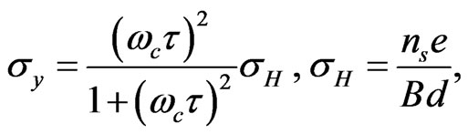
  are the number density and relaxation time of the electrons, respectively. However, Drude’s model was confronted with several problems. In Drude’s model electrons are distributed according to Maxwell-Boltzman distribution. Since electrons are fermions, Sommerfeld adopted a Fermi-Dirac distribution for electrons, and thus generalized the Drude’s model [2]. Electrons in conductors move on the surface which is two dimensional. Hall found that when a current passes in the x-direction of a conductor placed in a transverse magnetic field (along z-direction), the magnetic force forbids the movement of electrons across the y-axis. Charges are accumulated on the lateral sides of the conductor. The lateral potential difference divided by the horizontal current defines a transverse resistance that increases linearly with the magnetic field. This is known as Hall’s effect [3]. Since the motion of electrons in a conductor is generally twodimensional, a unified approach exhibiting this nature can be formulated using complex numbers. Such a formulation is shown recently to lead to interesting properties governing a two-dimensional system [4]. While dc conductivity is constant, ac conductivity varies with frequency. When a conductor is placed in a magnetic filed (B), Hall found that the conductivity along the y-direction varies with magnetic field. This magnetic conductivity is known as Hall’s conductivity,
 . It is given by
  [5]. At low temperature and high magnetic field, the Hall’s conductivity of a two-dimensional conductor is found to exhibit a plateau behavior and is independent of the applied magnetic field, viz.,
  where
where  is an integer [5]. Over the plateau regions the horizontal conductivity vanishes.
The discovery of the quantum Hall effect (QHE) boosted the interest in studying the magnetic properties of the two-dimensional systems. Of these magnetic properties in two-dimensions is the magnetic flux quantization. In fact, the magnetic flux quantization was first noticed by London and Onsager [6,7]. They showed that the flux embraced by the superconducting ring ought to be quantized in units of  [6,7]. They further inspired the suggestion that the quantization of the magnetic flux might be an intrinsic property of the electromagnetic field.
We express in this work the conductivity of conductors as a complex number with horizontal and vertical components. We further show that under low magnetic field, the horizontal conductivity reduces to the Drude’s conductivity, whereas the vertical component becomes vanishingly small. However, under high magnetic field the horizontal conductivity is less than the value suggested by Drude’s, while the vertical conductivity reduces to the Hall’s conductivity. In addition, we recently hypothesize a maximum conductivity for conductors, viz.
 [8]. The Hall’s conductivity is found to be equal to this maximum conductivity. Moreover, the quantum behavior of the two-dimensional Hall’s conductivity is found to be a signature of the quantization of the magnetic flux enclosed by the conductor. In two-dimensions, the Drude’s and Hall’s conductances are equal. This shows that the relaxation time of a two-dimensional conductor is about two orders of magnitudes bigger than the one in three dimensions.
2. Hall’s Conductivity
For a conductor with number density, n, the current density of the drifting electrons can be written as
 (1)
(1)
However, Ohm’s law states that
 (2)
(2)
where  is the conductivity of the material.
Write the current density, electric field and conductivity as
 (3)
(3)
Applying Equation (2) in (1), and equating the real and imaginary parts of the resulting equation, one gets
 (4)
(4)
The vanishing component of the y-component of Lorentz’s force yields
 (5)
(5)
Moreover, since there is no current flow along the y-direction, i.e.,  , Equations (1) and (4) yield
 (6)
(6)
and
 (7)
(7)
Hence, applying Equations (5)-(7) in (4) yields
 (8)
(8)
where  is the surface number density of the Hall surface, and
  is the conductor thickness. And since
  and
and , where
  is the conductor length (see Figure 1), Equations (6) and (8) become
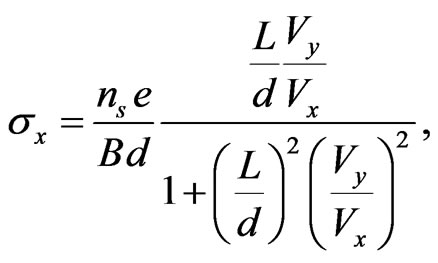 (9)
(9)
and
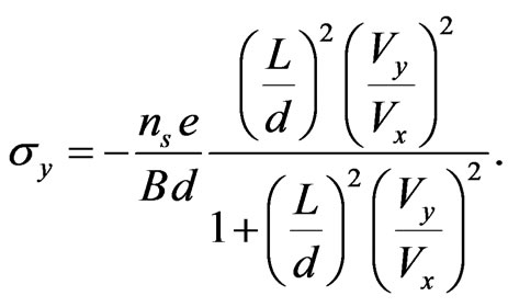 (10)
(10)
In steady state, the velocities of an electron with mass , in magnetic and electric fields, are governed by [2]
 (11)
(11)
where  and
and  are the cyclotron frequency and collision time, respectively. Since no current flow in the y-direction, then
 . Thus, Equation (11) yields
 (12)
(12)
Now substitute Equation (12) in Equations (6) and (8) to obtain
 (13)
(13)
and
 (14)
(14)
where  is the Hall’s conductivity. Now Equations (13) and (14) can be written as
 (15)
(15)
and
 (16)
(16)
where
 (17)
(17)
and  is the Drude’s conductivity. Thereforeas evident from Equation (15),
  is the zero-magnetic field dc conductivity. One can also introduce the electron mobility,
  in the above equations so that
  . It is remarkable that for low magnetic field or when
 reduces to the Drude’s conductivity of metals, i.e.,
  ,
,  and
and  . This shows that
  can be neglected (
 ). It is apparent from Equations (15) and (16) that when
 , then
  and
and  . This implies that
 , and hence,
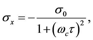
  can be neglected. We conclude that at low magnetic field, the vertical conductivity vanishes, and the conductor has only horizontal conductivity that is the Drude’s conductivity, viz.
 . Thus, for high magnetic field the horizontal conductivity vanishes, so that the material behaves like an insulator, and the vertical conductivity approaches Hall’s conductivity. We see that when
 one has
  and
and . This in fact occurs when
  attains its maximum value, as evident from Equation (16). Hence, at this state the two conductivities halved their maximum values. But at low temperatures and at high magnetic fields, the Hall’s conductivity exhibits plateaus where the conductivity becomes quantized in units of a multiple of
  [5]. In the plateau regions,
 . The variation of
  with the magnetic field is shown in Figure 2. Equation (15) can be seen as scaling the mass of the electron moving horizontally under a magnetic field, viz.,
  Thus, as we increase the magnetic field the electron mass increases making the horizontal conductivity exceedingly small. However, Equation (16) serves a scaling the mass of the electron moving vertically as,
Thus, the vertical mass of the electron decreases with increasing magnetic field, and hence, the vertical conductivity increases.
We can now define the xand y-resistivities as
 (18)
(18)
Using Equation (3), we obtain the two equations
 (19)
(19)
and
 (20)
(20)
Using Equations (15)-(17) one gets
 (21)
(21)
and
 (22)
(22)
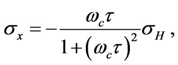
It is interesting to see that  is independent of the magnetic field, while
  does.
does.  is equal to the inverse of Drude’s conductivity, whereas
  is equal to the Hall’s conductivity. Consequently, the horizontal resistivity is independent of the magnetic field (but the
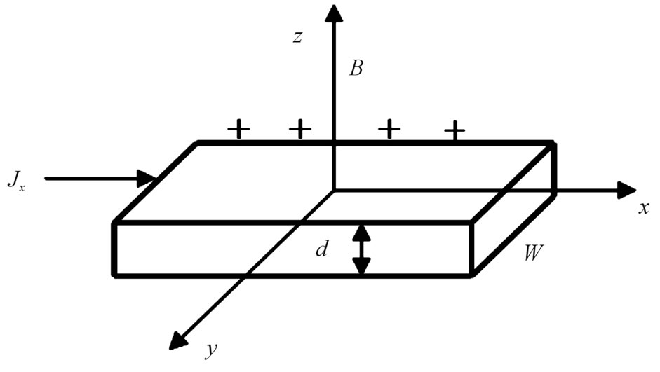
Figure 1. Hall’s bar setup shows the transverse magnetic field, B and longitudinal current, Jx.
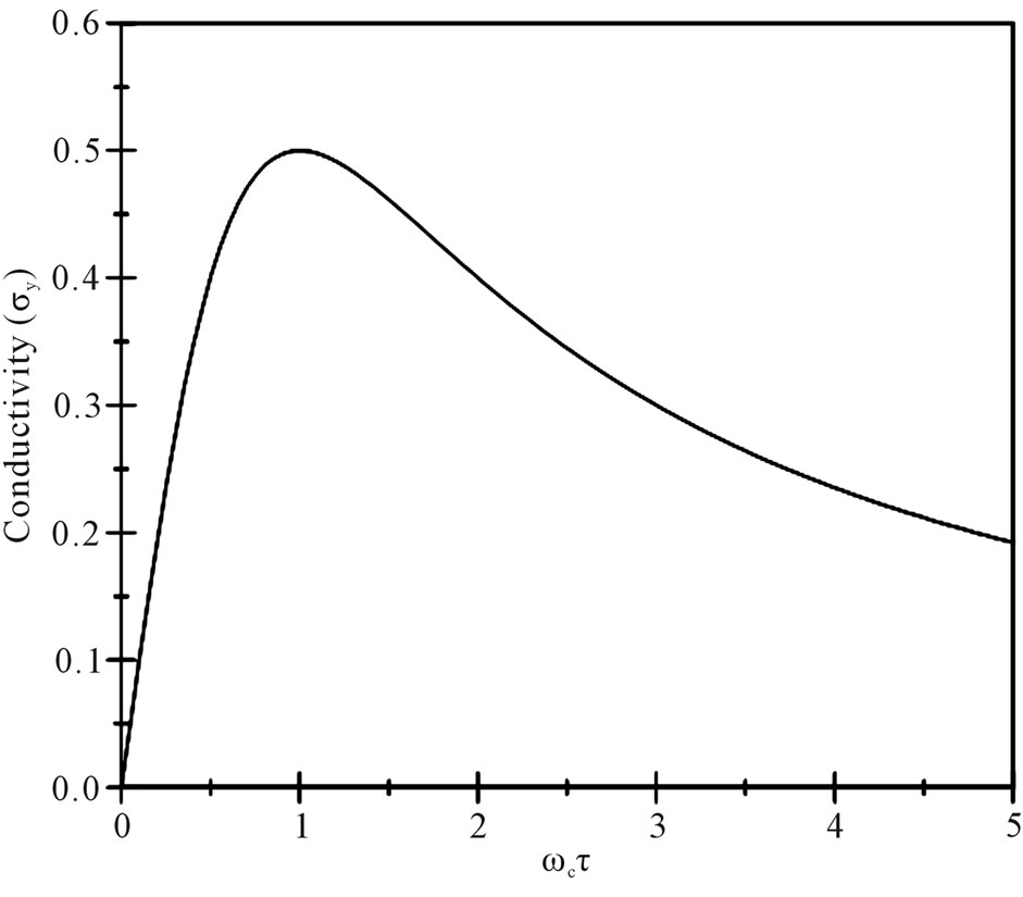
Figure 2. Variation of  (arbitrary scale) with the magnetic field
 . The maximum value of
  is
is .
.
corresponding conductivity does), while the vertical resistivity does.
Equations (19) and (20) reveal that  and
and  . It seems that this quantization occurs when the magnetic field is so high. Equation (13) shows that if
  is quantized then,
  is quantized too. It is apparent that
  follows a Lorentzian function of the cyclotron frequency. For a perfect conductor in a magnetic field,
  , so that
  and
and .
.
We have recently introduced a quaternionic mass where the bare mass can be expressed as a complex quantity, viz. [9],
 (23)
(23)
where  and
and  are the longitudinal and transverse masses, respectively. We may attribute
  and
and  to the mass of the electron when moving horizontally and vertically, respectively, across the conductor. The Drude’s conductivity,
  , is transformed into
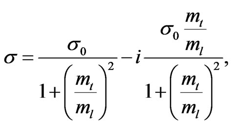 (24)
(24)
where  is the ordinary mass of the electron. Comparing this with Equations (15), (16) and (25) reveal that
 (25)
(25)
Therefore, in high magnetic field (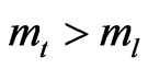 ) so that electrons move with a bigger mass in the transverse direction than in the horizontal direction, and vice versa.
Using Equation (14) the relaxation time can be written as
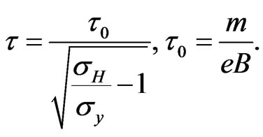 (26)
(26)
We remark that  is the relaxation time when
 , i.e., when
  is maximum. Moreover, when
  , then
 . It is evident that for a perfect conductor, i.e.,
  , then
 . We can thus define a perfect conductor in a magnetic field as the one with vertical conductivity equals to Hall’s conductivity.
When the magnetic field is so high (usually at low temperature) the horizontal current will vanish, and all electrons accumulated on the Hall sides of the conductor. The vertical conductivity will be equal to the Hall’s conductivity. Thus, the conductor behaves like an insulator horizontally and a perfect conductor vertically. In this case, one can calculated the displacement vector (
 ) inside the conductor. Notice that the Hall’s capacitance is given by
 , where
  is the width of the conductor,
  is the permittivity of the space between the two Hall’s surfaces, and the charge on the Hall side is
 . These yield
 (27)
(27)
where  is the lateral (Hall) surface number density.
3. Quantum Hall Effect
Let us now consider a two-dimensional conductor. In this case, . Now if we assume that
  is quantized [5], i.e.,
  , then Equations (13) and (16) dictate that both
  and
and  are quantized too. In twodimensions, the Drude and Hall conductances can be written as
 (28)
(28)
Therefore, Equation (17) now reads
 (29)
(29)
Hence,
 (30)
(30)
where N is the number of electrons and A is the crosssectional area of the sample (conductor). Note that the total flux encapsulated by the conductor, . Now if
  defines the quantum (unit) of flux, then
  gives the flux of N electron. Hence, Equation (30) defines the ratio (
 ) between the flux enclosed by the electrons and the total flux enclosed by the conductor. This implies that the total flux in the conductor is carried utterly by the electrons in the conductor. Thus, the total flux is quantized. Therefore,
  must be an integer.
 (31)
(31)
Equation (31) can be written as
 (32)
(32)
This is exactly the filling factor Klitzing et al. have obtained [5], but in a different way. In the quantum mechanical treatment,  represents the number of fully occupied Landau levels [5,10]. The degeneracy of the lowest Landau level is defined by
 . Equation (31) states that the magnetic field that gives rise to inter quantum Hall effect (IQHE) is the one such that the flux encapsulated by the conductor (area) is divided among the electron in such a way each electron carries a single flux quantum. But, other values of magnetic field don’t give rise to IQHE. Consequently, the magnetic flux is quantized, i.e.,
  , where
  is an integer. Thus, Equation (31) implies that
 . Therefore, there are more electrons than flux quanta. Hence, Hall’s conductivity stays constant unless the magnetic field satisfies the relation,
 . This latter relation defines the values of the magnetic field that drives the Hall’s conductivity to its next value.
We notice from Equation (29) that, in two-dimensions, Drude’s conductance is equal to Hall’s conductance provided the magnetic flux encircled by the conductor is a multiple of  Furthermore, it is interesting to deduce that the relaxation time in two-dimensions, with
  m−2, is
 . This is about two to three orders of magnitudes greater than that in three dimensions. The mean free path traversed by electrons in a conductor at room temperature, where electrons move with Fermi velocity, to be
  times that of the three dimensional conductors. In effect, one can regard the electron’s velocity as increased by this proportion while the relaxation time remains the same. As apparent from Equation (28), one can regard the electron mass to be lighter by this factor, i.e.,
 . This makes electrons appear to be quasi-relativistic. In such a case the Dirac’s equation should be used to describe electrons instead of the Schrödinger’s equation. Such a new situation is found to take place in graphene as demonstrated by Novoselov et al. [11].
Let us assume now that the thermal energy of the electrons is equal to the magnetic energy, i.e., . Hence, the condition when the vertical conductivity is maximum, i.e.,
  implies that
 , where
  is the Boltzman’s constant and T is the absolute temperature. This shows clearly the relaxation constant increases as temperature drops down. Therefore, the Drude’s conductivity varies inversely with temperature (
 ). For instance,
  when
when , and
, and , when
 . The latter case corresponds to a magnetic field of
 . This indicates that the Drude’s conductance (equals to Hall’s conductance) is very low temperature effect.
If we now assume that the angular momentum of the cyclotron motion is quantized, then , where s is an integer. This implies that the radius of the cyclotron motion is,
  , so that the flux enclosed is
 . Hence, the minimum flux an electron can encapsulate is
 . This coincides with the flux enclosed by a superconducting ring obtained by London and Onsager [6,7]. Notice that the magnetic length is defined as
  . Therefore, the cyclotron radius is a multiple of the magnetic length, i.e.,
 . Thus, for the first energy level (s = 1),
 .
.
4. Maximal Conductivity of Conductors
We have recently shown that the maximum conductivity of conductors ( ) is given by [8]
 (33)
(33)
If the Hall’s conductivity provides the maximum value of conductivity that any conductor can have, then equating these yields the number density
 (34)
(34)
Thus, Equation (34) gives . And since the number densities for typical conductors are in the range of
 , a magnetic field of
  is sufficient to provide such a limit! Remarkably, Equation (16) states the vertical resistivity has a limiting value which is the Hall’s conductivity. Hence, Hall’s conductivity represents the maximal conductivity of conductors.
5. Drude’s Ac Conductivity
In the case of finite frequency ( ), the Drude’s conductivity reads [2]
 (35)
(35)
The real and imaginary parts of  are then
 (36)
(36)
and
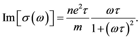 (37)
(37)
Apart from the minus sign, Equations (36) and (37) are the same as Equations (15) and (16) employing Equation (17) when the cyclotron frequency is equal to the source frequency, i.e., . Therefore, the electrons respond to the external frequency only when it is in resonance with the internal cyclotron frequency. Hence, the application of ac in a conductor is equivalent to the application of a transverse magnetic field. It seems that the static Hall conductivity evolves into the dynamical Hall conductivity. Moreover, the cyclotron frequency acts like a barrier (e.g., plasma frequency) below which no ac can influence the conductor. There could be drastic changes when this frequency is exceeded.
6. Concluding Remarks
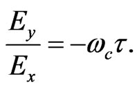
We have used a complex number to formulate the conductivities of conductors. We have shown that Drude’s and Hall conductivities are related by . Moreover, in two-dimensions the Drude’s and Hall’s conductances are equal, and the relaxation time is found to be
  times that for three dimensional conductors. The Hall’s conductivity for conductors is found to be equal to the maximal conductivity that we have recently hypnotized. Magnetic field changes appreciably the electric properties of conductors. Therefore, in the presence of magnetic field, the Drude, Hall and maximal conductivities are interrelated (unified). The Hall’s conductance is attributed to the flux quantization enclosed by the conductor.
7. Acknowledgements
I wish to thank Dr. H. M. Widatallah for useful discussion and enlightening. I would also like to thank Sultan Qaboos University (Oman) for inviting me in the framework of consultancy program, where this work is carried out.
REFERENCES
- P. Drude, Physikalische Zeitschrift, Vol. 1, 1900, p. 161.
- N. W. Ashcroft and N. D. Mermin, Solid State Physics, Prentice Hall, 1976.
- E. Hall, “On a New Action of the Magnet on Electric Currents,” American Journal of Mathematics, Vol. 2, No. 3, 1879, pp. 287-292. doi:10.2307/2369245
- A. I. Arbab, “The Complex Quantum Harmonic Oscillator Model,” Europhysics Letters, Vol. 98, No. 3, 2012, p. 30008. doi:10.1209/0295-5075/98/30008
- K. V. Klitzing, G. Dorda and M. Pepper, “New Method for High-Accuracy Determination of the Fine-Structure Constant Based on Quantized Hall Resistance,” Physical Review Letters, Vol. 45, No. 6, 1980, pp. 494-497. doi:10.1103/PhysRevLett.45.494
- F. London, “Superfuids,” Wiley, New York, 1950.
- L. Onsager, “Magnetic Flux through a Superconducting Ring,” Physical Review Letters, Vol. 7, 1961, p. 50. doi:10.1103/PhysRevLett.7.50
- A. I. Arbab, “On the Electric and Magnetic Properties of Conductors,” Advanced Studies in Theoretical Physics, Vol. 5, No. 9-12, 2011, pp. 595-604.
- A. I. Arbab, H. M. Widatallah and M. A. H. Khalafalla (Unpublished).
- L. D. Landau, “Paramagnetism of Metals,” Z. Phys., Vol. 64, 1930, pp. 629-637.
- K. S. Novoselov, A. K. Geim, S. V. Morozov, D. Jiang, Y. Zhang, S. V. Dubonos, I. V. Grigorieva and A. A. Firsov, “Electric Field Effect in Atomically Thin Carbon Films,” Science, Vol. 306, No. 5696, 2004, pp. 666-669.