Applied Mathematics
Vol.4 No.12(2013), Article ID:41159,5 pages DOI:10.4236/am.2013.412236
On the Markov Chain Binomial Model
1Department of Mathematics and Statistics, Grant MacEwan University, Edmonton, Canada
2Department of Mathematics and Statistics, University of Saskatchewan, Saskatoon, Canada
Email: IslamM@macewan.ca, oshaughn@math.usask.ca
Copyright © 2013 M. N. Islam, C. D. O’shaughnessy. This is an open access article distributed under the Creative Commons Attribution License, which permits unrestricted use, distribution, and reproduction in any medium, provided the original work is properly cited.
Received May 15, 2013; revised June 15, 2013; accepted June 23, 2013
Keywords: Extrabinomial Variation; Markov Chain Binomial Model; Maximum Likelihood Estimation; Sequence Data
ABSTRACT
Rudolfer [1] studied properties and estimation of a  state Markov chain binomial (MCB) model of extra-binomial variation. The variance expression in Lemma 4 is stated without proof but is incorrect, resulting in both Lemma 5 and Theorem 2 also being incorrect. These errors were corrected in Rudolfer [2]. In Sections 2 and 3 of this paper, a new derivation of the variance expression in a setting involving the natural parameters
 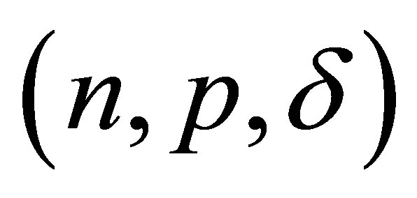 is presented and the relation of the MCB model to Edwards’ [3] probability generating function (pgf) approach is discussed. Section 4 deals with estimation of the model parameters. Estimation by the maximum likelihood method is difficult for a larger number n of Markov trials due to the complexity of the calculation of probabilities using Equation (3.2) of Rudolfer [1]. In this section, the exact maximum likelihood estimation of model parameters is obtained utilizing a sequence of Markov trials each involving n observations from a
  state MCB model and may be used for any value of n. Two examples in Section 5 illustrate the usefulness of the MCB model. The first example gives corrected results for Skellam’s Brassica data while the second applies the “sequence approach” to data from Crouchley and Pickles [4].
1. Introduction
Let  be a stationary two-state Markov chain with states 0 (failure) and 1 (success), an initial probability distribution denoted
  in which
  and
and , and transition probabilities
  for
for 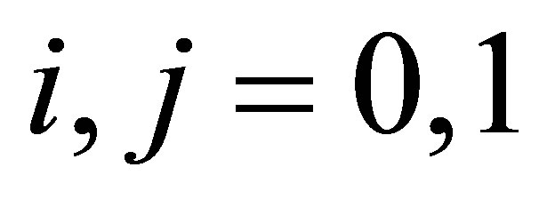 and
and  represented in a transition probability matrix
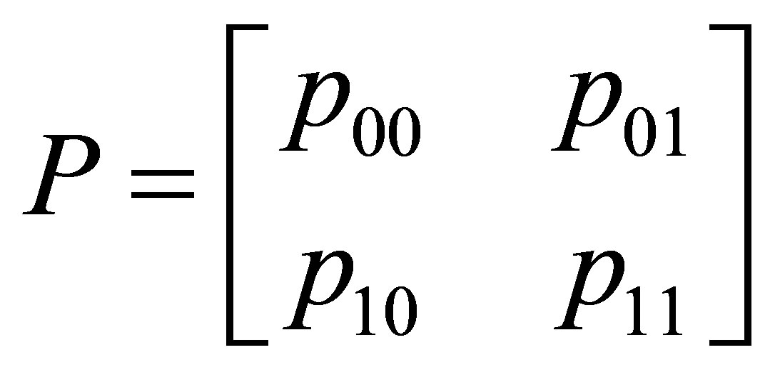 . (1)
. (1)
If  is a sequence from a
  state Markov chain, let
 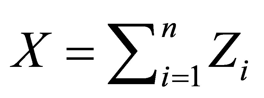 denotes the number of successes in n Markov trials. The random variable X may be said to have a Markov chain binomial (MCB) distribution with parameters n and p, and transition matrix P.
Rudolfer [1] studied properties and estimation for this 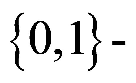 state Markov chain binomial model. A formula for computing the probabilities
  is given as his Equation (3.2), and an expression for the variance of X is given as Equation (3.4) in his Lemma 4. However, the variance expression is incorrect and hence Lemma 5 and Theorem 2 are also incorrect. These results were corrected in Rudolfer (2). Section 3 of this paper provides an alternative derivation of the correct versions of these results.
Even for relatively small values of n, computation of the probabilities 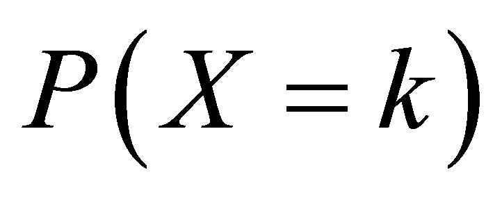 using Rudolfer’s Equation (3.2) involves tedious summations making maximum likelihood estimation for the model difficult. Using the Edwards’ [3] formulation and an approach introduced by Devore [5] and results given by Edwards [6], exact maximum likelihood estimation of model parameters is obtained in Section 4 using a sequence of observations assumed to come from a
  state Markov chain with the transition probability matrix P given in (1) above.
Two examples are presented in Section 5 to illustrate the effect of the corrections and of parameter estimation utilizing the sequence nature of the data.
2. The Markov Chain Binomial Model
Rudolfer [1] writes the matrix of transition probabilities (1) for the  state Markov chain as
 (2)
(2)
in which . For such a chain, the probability of a success at stage
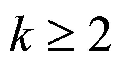 ,
,  , depends on k and the initial probability distribution
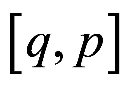 . This is seen by noting that, for
 ,
,
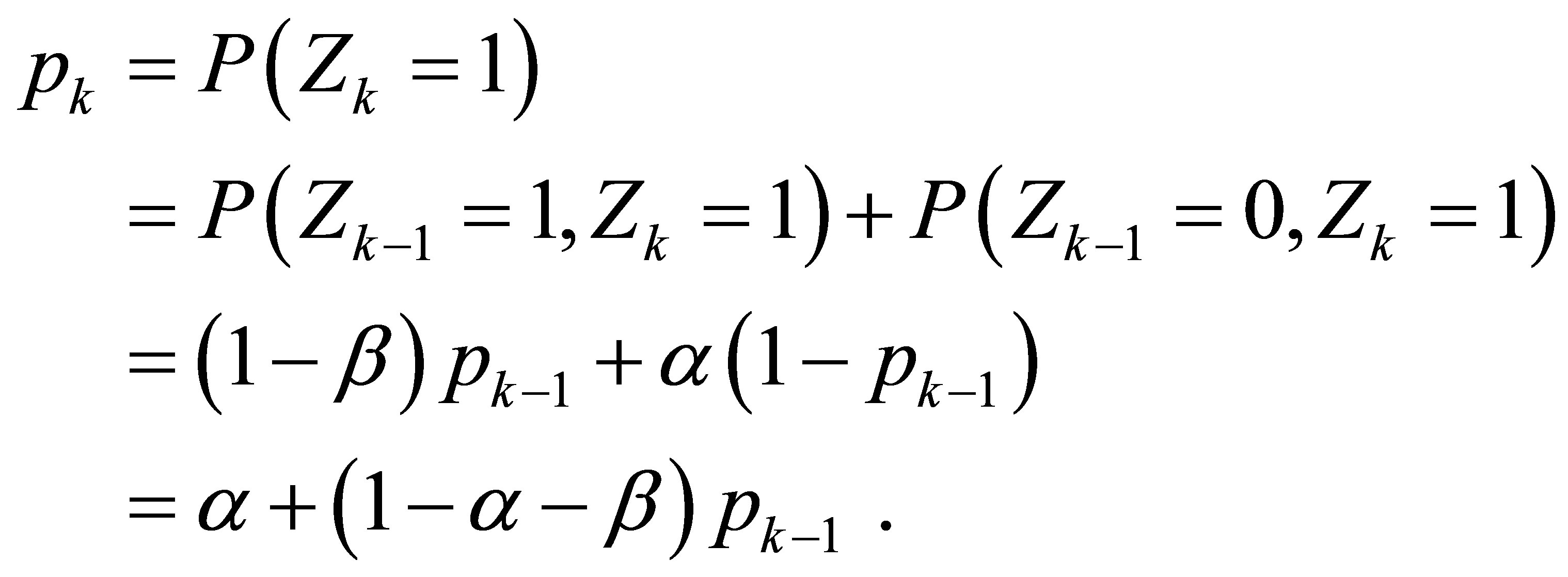
Recursive application of this procedure results in
 .
.
Since  it follows that, as
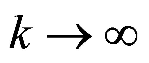 ,
, 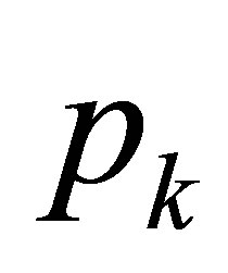 tends to the limit
 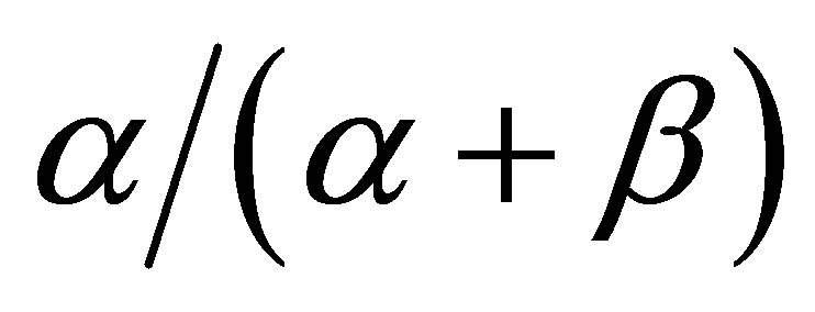 independent of the initial state (0 or 1) and of the initial probability distribution
 . Also, if the initial probability distribution has
 , the probability of a success
  is constantly equal to
  throughout all trials.
If the probability of success at the first trial is  so that
  , and if
 , then the transition matrix (2) can be written as
 . (3)
. (3)
Replacing Rudolfer’s [1] parameter ![]() with r, the transition matrix (3) is seen to be equivalent to the one for the MCB model in Edwards [3]. The parameter
with r, the transition matrix (3) is seen to be equivalent to the one for the MCB model in Edwards [3]. The parameter ![]() in Rudolfer [1] has the same interpretation as that of r in Edwards [3], namely it is the first-order autocorrelation between
in Rudolfer [1] has the same interpretation as that of r in Edwards [3], namely it is the first-order autocorrelation between 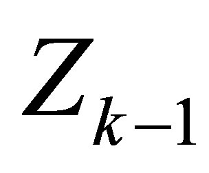 and
and 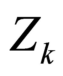 for
for . Thus, Rudolfer’s and Edwards’ MCB models are exactly the same probability model under re-parameterization with parameters n, p and
![]() , and transition matrix P as given in (3). A random variable X with this distribution may be denoted by
, and transition matrix P as given in (3). A random variable X with this distribution may be denoted by .
.
Edwards’ [3] approach involved the use of the probability generating function (pgf). For given n, the pgf of the MCB model is
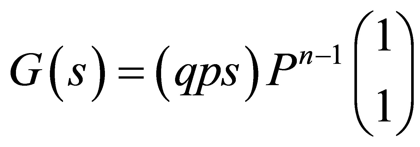 (4)
(4)
in which s is a dummy variable. Explicit expressions for the probabilities  can be obtained from the pgf (4), although the calculations are not straightforward. For example, in the case of n = 3, the probabilities are

These equations can also be obtained by substituting  and
and  into the expressions for the probabilities as given by Rudolfer [1] at the beginning of Section 4.2 of his paper.
3. Rudolfer’s [1,2] Corrected Results
Rudolfer’s [1] Lemma 4 incorrectly expresses the variance of a random variable  as
as

resulting in an incorrect statement of his Lemma 5 and thus Theorem 2. In Rudolfer [2] the variance expression is corrected and proper statements of Lemma 5 and Theorem 2 are given. A corrected version of Lemma 4 is presented with an alternative derivation, and is followed by the corrected Theorem 2.
Corrected Lemma 4 of Rudolfer [1]
For a random variable  with
with  and
and , the mean and variance are
 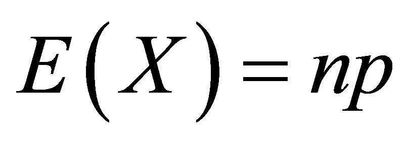 and
and
 (5)
(5)
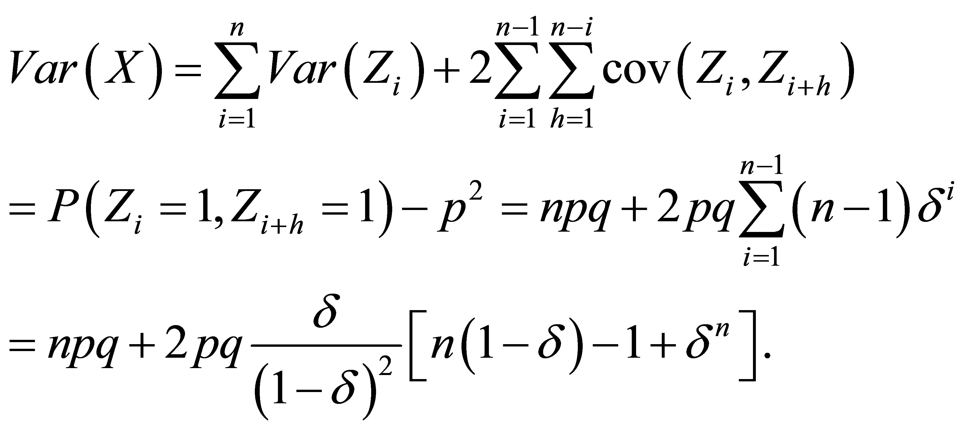
Proof: The n-th step transition probability matrix is equal to
 (6)
(6)
as is easily shown by diagonalizing the transition matrix P given in (3), using its right and left eigenvectors and its eigenvalues. For  and
and , it follows from (6) that

and thus
Corrected Theorem 2 of Rudolfer [1]
For 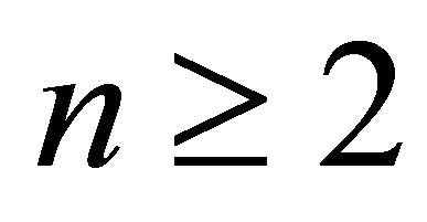 and
and ,
,

where .
.
Proof: From the variance expression (5), let
 (7)
(7)
From (7) it follows that

which immediately gives the result in the theorem.
4. Estimating the Model
Consider N trials from a  state Markov chain with parameters n, p and
![]() . Let
. Let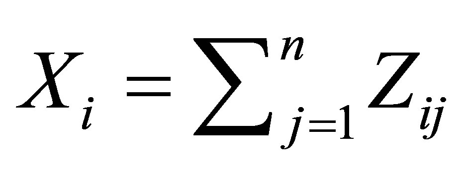 . Then
  are independent, identically distributed random variables each having the MCB distribution with parameters n, p and
![]() .
.
4.1. Moment Estimation of p and 
Let  be a random sample of size N from the
  distribution, and let
  and
and  be the sample mean and sample second raw moment respectively. Using the method of moments, estimators
 ![]() and
and ![]() are determined as solutions to the equations
are determined as solutions to the equations
 (8)
(8)
and
 (9)
(9)
Equation (8) gives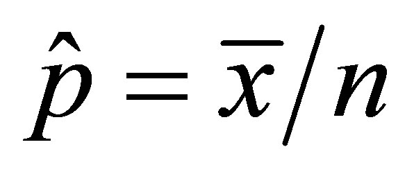 . Replacing p by
 ![]() in Equation (9) and rearranging gives
in Equation (9) and rearranging gives

This nonlinear equation can be solved for ![]() by iteration using MAPLE or other mathematical software.
by iteration using MAPLE or other mathematical software.
4.2. Maximum Likelihood Estimation of p and  for Sequence Data
Even for a relatively small value of n, maximum likelihood estimation of the model parameters p and ![]() may prove to be difficult using either Rudolfer’s [1] Equation (3.2) (in this case, the summation in the expression for the probabilities is complex) or Edwards’ [3] pgf approach. However, if N sequences
may prove to be difficult using either Rudolfer’s [1] Equation (3.2) (in this case, the summation in the expression for the probabilities is complex) or Edwards’ [3] pgf approach. However, if N sequences  each involving n trials from a
  state Markov chain with transition matrix (1) are observed, an alternative approach to obtaining maximum likelihood estimates of the parameters p and
 ![]() is as follows.
is as follows.
The likelihood function for such sequence data can be written in the form
 (10)
(10)
in which  is the number of the N sequences that begin with the occurrence of state 1 (that is, success),
  is the number of sequences that begin with the occurrence of state 0 (that is, failure), and
  denotes the total number of transitions from state i to state j observed within the N sequences. Since each of the N sequences involves n trials, a total of nN transitions will be observed. If the transition probabilities are written in terms of p,
 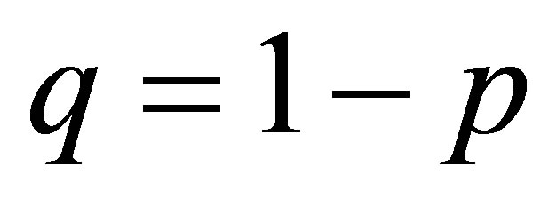 and
and ![]() as in the version of the transition matrix P in expression (3), the likelihood function (10) becomes
as in the version of the transition matrix P in expression (3), the likelihood function (10) becomes
 (11)
(11)
Devore [5] obtained maximum likelihood solutions by ignoring the contribution of the initial state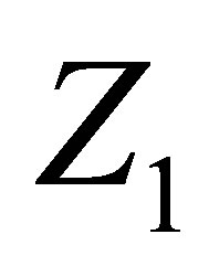 , and considering only the modified likelihood function
 (12)
(12)
The solutions obtained restricting attention to this modified likelihood function are
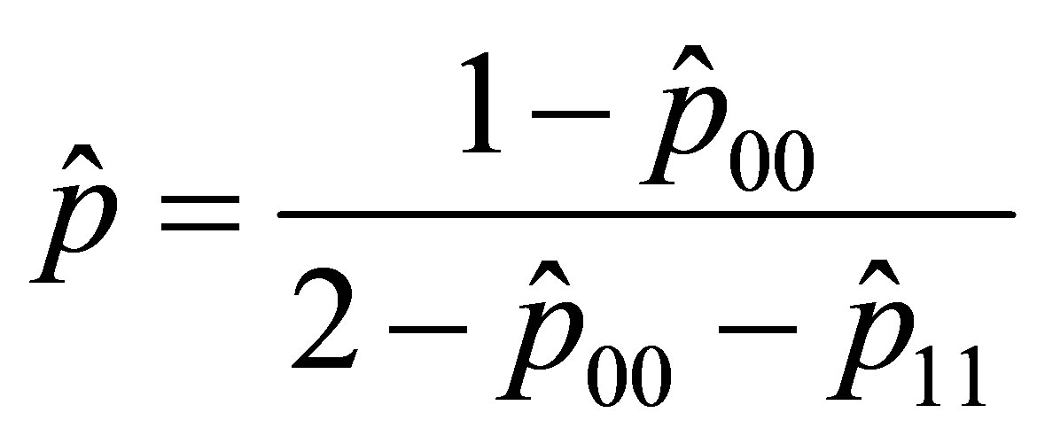 (13)
(13)
 (14)
(14)
in which  and
and  .
.
Edwards [6] provides a solution using the full likelyhood function (11). Equating each of the partial derivatives 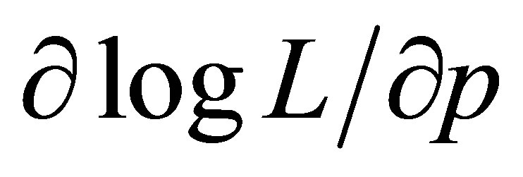 and
and 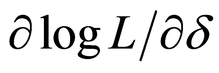 of the log-likelihood function to zero and solving for
 ![]() provides the two expressions
provides the two expressions
 (15)
(15)
and
 (16)
(16)
Equating expressions (15) and (16), and letting ,
,  ,
,  and
and  results in the cubic equation in p
 (17)
(17)
which can be solved by standard methods. Substituting the solution ![]() from (17) into either (15) or (16) provides the solution
from (17) into either (15) or (16) provides the solution![]() .
.
5. Examples
5.1. Application to Skellam’s [7] Brassica Data
Rudolfer [1,2] used the “Brassica” data of Skellam [7] to illustrate the model and parameter estimation. Using this data and the method of moments with result (5) of the corrected Lemma 4, the obtained estimate  is essentially the same as the maximum likelihood estimate
 . The corrected moment Equation (9) for the variance in the case of n = 3 is
 (18)
(18)
On substitution of , the quadratic Equation (18) gives the possible root
 , rejecting the other root as it is less than
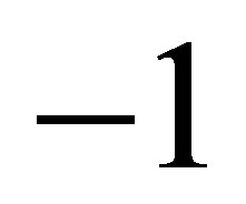 .
.
Comparisons of the p-values and of the values of the Chi-square statistics given in Table 1 suggest that the Markov chain binomial model fitted by the method of moments using the corrected variance Formula (5) gives a fit very similar to those provided by the maximum likelihood method in Rudolfer [1] and the corrected method of moments method in Rudolfer [2].
5.2. Application to Human Birth-Order Data
Using the solutions provided by Devore’s [5] modified likelihood function and by Edwards’ [6] full likelihood function, the MCB model is fitted to a case in which a sequence of observations is given. Table 2 gives birthorder data for families with four children from Finland and from the United States. This data appears in Crouchley and Pickles [4]. It is assumed that the data are generated by a Markovian dependent sequence as defined in (1). The parameters p and ![]() are the quantities of interest in the analysis.
are the quantities of interest in the analysis.
Let state 0 refer to females and state 1 to males. For the Finish data, the full likelihood function, as given by (10) and then (11), is
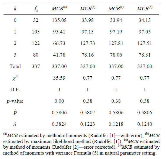
Table 1. Fits of the MCB model to Skellam’s [7] Brassica data.

Table 2. Frequencies of birth-order for families of four children from Finland and the United States.

From the latter form, the maximum likelihood estimates are determined to be  and
and  , and the estimated matrix of transition probabilities is

Using Devore’s [5] modified likelihood function (12), the estimated matrix of transition probabilities is

from which, applying Equations (13) and (14),  and
and .
.
Similarly, for the case of the United States population the estimated parameters from the full likelihood function are  giving as the estimated matrix of transition probabilities

Using Devore’s method, the estimated matrix of transition probabilities is

so that  and
and .
.
6. Discussion
In the application of the Markov chain binomial model to the Brassica data of Skellum [7] using the method of moments, Table 2 illustrates that the variance expression (5) results in a fit little different from that provided by the method of moments using Rudolfer’s [2] corrected values.
The second example dealing with birth-order data presented in Crouchley and Pickles [4] illustrates the usefulness of the “sequence data approach” in finding maximum likelihood estimates for the MCB model. Very little difference is seen in the estimates in this approach between using the full likelihood equation solution discussed by Edwards [6] and using the modified likelihood equation as discussed by Devore [5].
REFERENCES
- S. M. Rudolfer, “A Markov Chain Model of Extrabinomial Variation,” Biometrika, Vol. 77, No. 2, 1990, pp. 255-264. http://dx.doi.org/10.1093/biomet/77.2.255
- S. M. Rudolfer, “Correction to a Markov Chain Model of Extrabinomial Variation,” Biometrika, Vol. 78, No. 4, 1991, p. 935. http://dx.doi.org/10.2307/2336950
- A. W. F. Edwards, “The Meaning of Binomial Distribution,” Nature (London), Vol. 186, 1960, p. 1074. http://dx.doi.org/10.1038/1861074a0
- R. Crouchley and A. R. Pickles, “Methods for the Identification of Lexian, Poisson and Markovian Variations in the Secondary Sex Ratio,” Biometrics, Vol. 40, No. 1, 1984, pp. 165-175. http://dx.doi.org/10.2307/2530755
- J. L. Devore, “A Note on the Estimation of Parameters in a Bernoulli Model with Dependence,” Annals of Statistics, Vol. 4, No. 5, 1976, pp. 990-992. http://dx.doi.org/10.1214/aos/1176343597
- A. W. F. Edwards, “Estimation of the Parameters in Short Markov Sequences,” Journal of the Royal Statistical Society, Series B, Vol. 25, No. 1, 1963, pp. 206-208.
- J. G. Skellam, “A Probability Distribution Derived from the Binomial Distribution by Regarding the Probability of Success as Variable between the Sets of Trials,” Journal of the Royal Statistical Society, Series B, Vol. 10, No. 2, 1948, pp. 257-261.

