Applied Mathematics
Vol.3 No.12A(2012), Article ID:26099,4 pages DOI:10.4236/am.2012.312A298
Server Workload in an M/M/1 Queue with Bulk Arrivals and Special Delays
1Department of Mathematics & Statistics, University of Windsor, Windsor, Canada
2Department of Management Science, University of Windsor, Windsor, Canada
Email: brill@uwindsor.ca, hlynka@uwindsor.ca
Received November 10, 2012; revised December 10, 2012; accepted December 17, 2012
Keywords: M/M/1 Queue; Bulk Arrivals; Delay before Joining; Workload; Integral Equations; Level crossing Method
ABSTRACT
We consider a variant of M/M/1 where customers arrive singly or in pairs. Each single and one member of each pair is called primary; the other member of each pair is called secondary. Each primary joins the queue upon arrival. Each secondary is delayed in a separate area, and joins the queue when “pushed” by the next arriving primary. Thus each secondary joins the queue followed immediately by the next primary. This arrival/delay mechanism appears to be new in queueing theory. Our goal is to obtain the steady-state probability density function (pdf) of the workload, and related quantities of interest. We utilize a typical sample path of the workload process as a physical guide, and simple level crossing theorems, to derive model equations for the steady-state pdf. A potential application is to the processing of electronic signals with error free components and components that require later confirmation before joining the queue. The confirmation is the arrival of the next signal.
1. Introduction
The M/M/1 arrival/delay mechanism considered in this paper was introduced by Hlynka [1], who derived the Laplace transform of the busy period of the server, using the probabilistic interpretation of the Laplace transform. The busy period in that analysis included the idle times of the server while a secondary is being delayed.
Here we analyze the model using a level crossing approach, and derive: the steady-state pdf of the server workload; probability that the system is empty; probability that the server is idle when a secondary is being delayed; expected busy period (as defined in Hlynka [1]); a stability condition; expected time the server is busy in a cycle between instants of system emptiness, or between instants the server becomes idle and a secondary is being delayed. An advantage of the level crossing method used here is that it focuses on the workload process in a concrete manner. That is, it uses physical properties of a typical sample path of the workload process as a guide, and simple level crossing theorems, to formulate the model equations for the key probability distributions of the model. Viewing the sample path in this concrete manner, makes the solution procedure intuitive, straightforward, and suggestive of future research ideas.
Section 2 specifies the M/M/1 variant and sample path structure. Section 3 derives the model equations for the steady-state pdf of the workload, and specifies related quantities. Section 4 uses the model equations to obtain relevant constant terms, and gives a numerical example of the steady-state pdf of workload.
2. The M/M/1 Variant
Singles (primaries) arrive at the system at Poisson rate  and pairs (pair = primary + secondary) arrive at the system at Poisson rate
 ; let
; let . When a primary arrives at the system, it immediately joins the M/M/1 queue, either alone or just behind a secondary that was being delayed. When a secondary arrives at the system it splits from its primary and is delayed in a separate area outside the queue. The delayed secondary is “pushed” by the next arriving primary to join the queue, followed immediately by the new primary. (Thus the delay of each secondary before joining the queue is distributed as exponential-
![]() .) Customers in the queue are served one at a time at exponential rate
.) Customers in the queue are served one at a time at exponential rate  in firstcome-first-served order. When a primary joins the queue alone, the server workload is increased by exponential-
 . When a primary and secondary join the queue simultaneously, the server workload is increased by Erlang (2,
 ), i.e., the sum of two independent exponential-
 ’s. All secondaries join the queue simultaneously with (next) primaries. The number of secondaries being delayed in the system at any instant is either 0 or 1.
Define the state of the system as 
where W(t) = server workload at time ,
,  if zero secondaries are being delayed,
  if one secondary is being delayed. The state with zero customers in the system is denoted by
 . The state when the server is idle and one secondary is being delayed is denoted by
 . Let
. Let  denote an exponential-
 random variable, and
  denote an Erlang
 random variable.
2.1. Sample Path of 
Technique of “Lines and Sheets (or Pages)” We utilize a technique of “lines and sheets (or pages)” to picture the state space and a sample path in it (e.g., see Brill [2] Section 4.6). This technique partitions the state space into mutually exclusive and exhaustive physical lines and sheets corresponding to the states of .
.
We select an arbitrary continuous subset in each sheet, having one boundary as a fixed level ![]() in the state space of
in the state space of , e.g.,
  ,
, . We use this concrete physical picture as a guide to balance the samplepath exit and entrance rates of the selected state-space subsets. Simple level-crossing theorems (e.g., Brill [2]) guarantee that the partial steady-state pdf of
  for each sheet is a unique term, or linear factor in a term, of the corresponding balance equation. The balance equations are generally Volterra integral equations of the second kind with parameter. Thus there is an isomorphism between the physical sample path structure and the model equations.
Consider the sample path of  in Figure 1. All jumps due to an arrival on page 0 are distributed as
  because only primaries join the queue when arrivals find zero delayed secondaries present. All jumps due to an arrival on page 1 are distributed as
  because both the delayed secondary and the arriving primary join the queue simultaneously.
2.2. Description of the Sample Path of  in Figure 1
At time 0 the system is empty (state ). A single arrives and the SP (sample path) jumps to level
  on page 0; the arrival immediately starts service. The SP decreases at rate
  A pair arrives, the primary joins the queue and the secondary is delayed; the SP jumps
  since the server workload includes only those customers in the queue, and transits to page 1 (delayed secondary present).
A single arrives and pushes the delayed secondary to join the queue; the single joins just after it. The SP jumps  and transits to page 0 (no delayed secondary present).
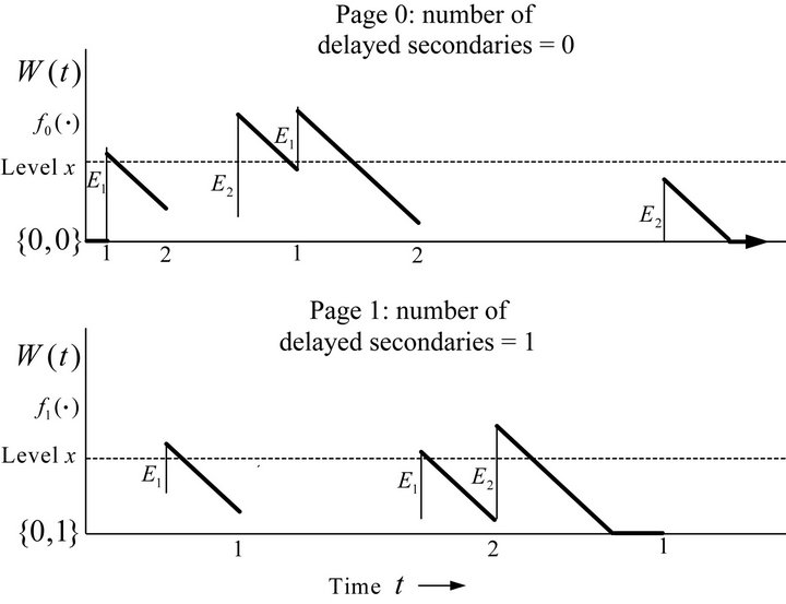
Figure 1. A sample path of .
.
A single arrives and joins the queue; the SP jumps  and remains on page 0. A pair arrives; the primary joins the queue and the split-off secondary becomes delayed. The SP jumps
  and transits to page 1. A pair arrives, the primary pushes the delayed secondary into the queue and joins just after it; the new secondary becomes delayed. The SP jumps
  and remains on page 1. The SP hits level 0 from above, and remains in state
  for a time distributed as exponentia-
![]() (server idle). A single arrives, pushes the delayed secondary into the queue and follows just after it. The SP jumps by
(server idle). A single arrives, pushes the delayed secondary into the queue and follows just after it. The SP jumps by  and transits to page 0. Finally the SP hits level 0 from above and enters
  (system empty).
Figure 1 illustrates a cycle starting and ending in state . A cycle starting and ending in state
  would be produced similarly.
3. Equations for Probability Distribution of Server Workload

Guided by the sample path (Figure 1) we write a system of balance equations for the singleton states  and
and , and for sets of continuous states
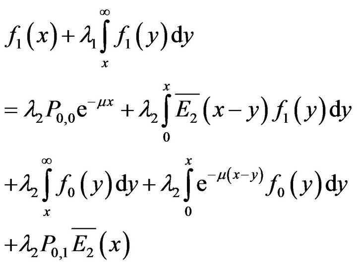
 . Explanations of the equations are given immediately after Equation (5).
State 
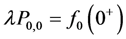 (1)
(1)
State 
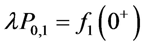 (2)
(2)
States 
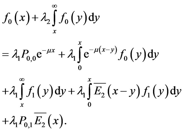 (3)
(3)
States 
 (4)
(4)
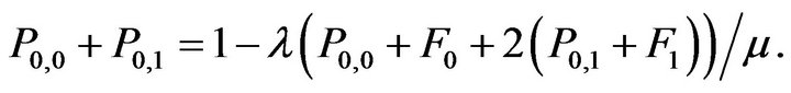
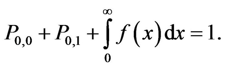
Total Probability = 1
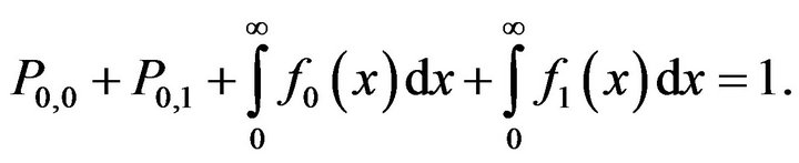 (5)
(5)
Explanation of Equations (1)-(5)
Equation (1): Left side = (exit rate of ). Right side = (downcrossing rate of level 0 on page 0) = (rate at which system is emptied).
Equation (2): Left side = (exit rate of ). Right side = (downcrossing rate of level 0 on page 1).
Equation (3): Left side = (exit rate of ) due to: i) (downcrossings of level
 ![]() on page
on page ) + ii) (arrivals of pairs). Right side = (entrance rate of
 ) due to: i) (singles arriving to an empty system bringing a workload
![]() ) + ii) (singles arriving when the state is
) + ii) (singles arriving when the state is  bringing a workload
 , summed for
 ) + iii) (singles arriving when the state is in
 ) + iv) (singles arriving when the state is
  adding a workload
  summed on
 ) + v) (singles arriving when the state is
  adding a workload
![]() ).
).
Equation (4): Similar reasoning as for Equation (3).
Equation (5): Sum of probabilities = 1.
Related Quantities
We now consider related quantities obtainable from the solution of Equations (1)-(5):  = proportion of time the system is empty;
  = proportion of time the server is idle and a delayed secondary is present;
 = proportion of time the server is busy and no delayed secondary is present;
  =
=
proportion of time the server is busy and a delayed secondary is present.
Let  time between successive
  entrances into state
  (system becomes empty).
Let  time between successive
  entrances into state
  (server becomes idle and a delayed secondary is present). Then
  and
and  are regenerative cycles of regenerative processes. From the elementary renewal theorem and (1) and (2)
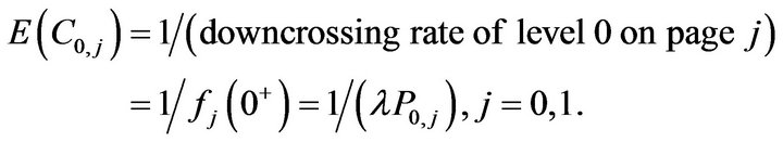 (6)
(6)
Let  be the total time that the server is busy during a cycle
 . (Note that
  is composed generally of non-contiguous time segments.) By the theory of regenerative processes (e.g., Cohen [3]) and (6)

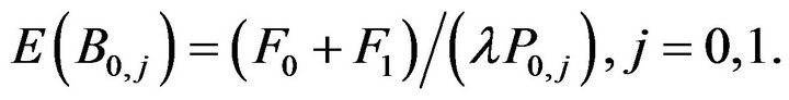 (7)
(7)
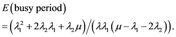
If we define a “busy period” as the proportion of  such that there is at least one customer in the system as in Hlynka [1] (which includes the time that the server is idle while a delayed secondary is present), then
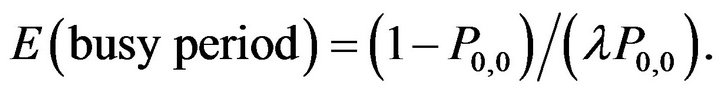 (8)
(8)
4. Relevant Constants and Numerical Example of Steady-State PDF of Workload
4.1. Relevant Constants
Before solving for  and
and
 , we solve six linearly independent equations for the constants
 The first two equations are (1)
and (2). The second two equations are obtained by letting  in (3) and (4). The fifth equation is (5).
The sixth equation is obtained by considering the system from the server’s point of view. The arrival rate to the queue is 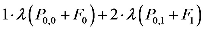 since only the arriving primary joins when zero delayed secondaries are present, and two join (arriving primary + present delayed secondary) when one secondary is present. The steady-state probability that the server is idle is
  (long-run traffic intensity) =
 . The server does not distinguish between idle periods when a delayed secondary is present or is not present. Thus
  (server is idle)
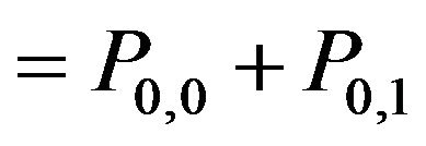 . This yields the sixth equation
 (9)
(9)
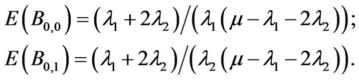
Solving the six equations gives the four quantities (as well as ):
):
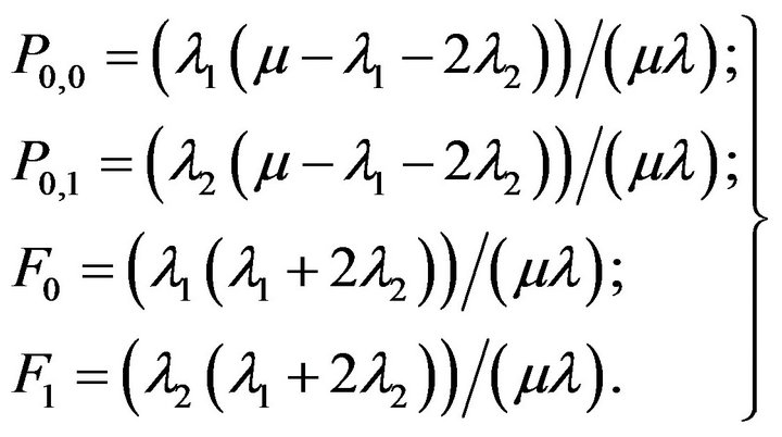 (10)
(10)
From (7)
 (11)
(11)
From (8)
 (12)
(12)
At least one of  must be positive for a steady state distribution to exist. This implies that
 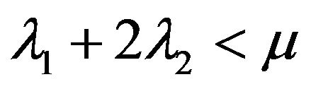 is the condition for stability, which agrees with intuition.
Note that if  the system behaves like a standard
  queue. If
  it behaves like a standard
  queue with regard to the workload.
4.2. Numerical Example of Steady-State PDF of Server Workload
We obtain formulas for  and
and  by computing Laplace transforms and inverting them, with the aid of Maple software. Let
  denote the Laplace transform of
 . We take Laplace transforms on both sides of (3) and (4) and solve two linear equations for
 . Taking the inverse Laplace transforms and adding gives the steadystate pdf
 . The analytical expressions obtained are lengthy, and are not shown here.
We present a numerical example with arbitrary parameter values , which illustrates typical results.
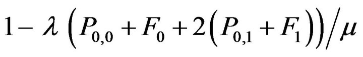
The steady-state pdf of workload is (see Figure 2)
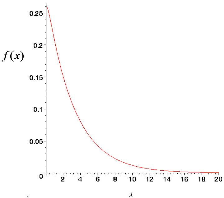
Figure 2. Plot of steady-state pdf f(x) using the parameter values in Subsection 4.2.
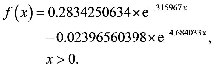 (13)
(13)
Also
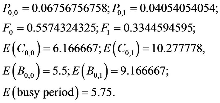
Note that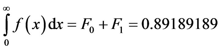 ;
;
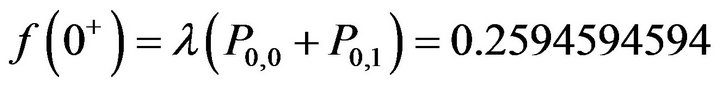 ;
;
5. Acknowledgements
This work was supported by the Natural Sciences and Engineering Research Council of Canada.
REFERENCES
- M. Hlynka, “An M/M/1 Queue with Bulk Arrivals and Delays,” Canadian Operational Research Society Conference Presentation, Niagara Falls, June 2012.
- P. H. Brill, “Level Crossing Methods in Stochastic Models,” Springer, New York, 2008. doi:10.1007/978-0-387-09421-2
- J. W. Cohen, “On Regenerative Processes in Queueing Theory,” Lecture Notes in Economics and Mathematical Systems, Spring-Verlag, New York, 1976.