Applied Mathematics
Vol.3 No.11(2012), Article ID:24543,11 pages DOI:10.4236/am.2012.311239
Trajectory Controllability of Nonlinear Integro-Differential System—An Analytical and a Numerical Estimations*
1Mallory Hall, Virginia Military Institute, Lexington, USA
2Roop Hall, James Madison University, Harrisonburg, USA
Email: #charlishajardn@vmi.edu, chalishd@jmu.edu, davidja@vmi.edu
Received September 4, 2012; revised October 8, 2012; accepted October 15, 2012
Keywords: Trajectory Controllability; Monotone Operator Theory; Set Valued Function; Lipschitz Continuity; Finite Difference; Optimization
ABSTRACT
A stronger concept of complete (exact) controllability which we call Trajectory Controllability is introduced in this paper. We study the Trajectory Controllability of an abstract nonlinear integro-differential system in the finite and infinite dimensional space setting. We will then discuss how approximations to these problems can be found computationally using finite difference methods and optimization. Examples will be presented in one, two and three dimensions.
1. Introduction
The concept of controllability (introduced by Kalman, 1960) leads to some very important conclusions regarding the behavior of linear and nonlinear dynamical systems. Most of the practical systems are nonlinear in nature and hence the study of nonlinear systems is important. There are various notions of controllability such as complete controllability [1], approximate controllability [2], exact controllability [3-7], partial exact controllability [8], null controllability [9], local controllability [10], constrained controllability [11,12] and references cited in. A new notion of controllability, namely, Trajectory controllability (T-controllability) is introduced here for some abstract nonlinear integro-differential systems. In T-controllability problems, we look for a control which steers the system along a prescribed trajectory rather than a control steering a given initial state to a desired final state. Thus this is a stronger notion of controllability.
T-controllability problems for nonlinear integro and partial differential equations (PDE)s also offer a challenging computational problem. These parabolic problems generally require a more complicated implicit method for the numerical algorithm to be robust under different discretizations instead of the simpler explicit discretizations. n addition to offering varying challenges on how to accurately solve the PDEs for a given control, the problems also offered various challenges in how to optimize for the T-control. Assuming n control points per dimension, the discretized problem is an optimization problem in  in two dimensions and
  which can become computationally difficult quickly. We employed both gradient and non-gradient based approaches to solving these optimization problems.
Under suitable conditions, the T-controllability of nonlinear system in finite dimensional case has been established in Section 2. Then the result is extended to infinite dimensional case in Section 3. We use the tools of monotone operator theory and set-valued analysis. We also use Lipschitzian and monotone nonlinearities with coercivity property in Section 3. In Section 4 we discuss how to approximate the solutions to these problems using finite difference discretization and numerical optimization. Examples are provided to illustrate our results.
REMARK 1.1. In practical applications, controls are always in some sense of constrained. Recently Klamka [12] studied the sufficient conditions for constrained local relative controllability of semilinear ordinary differential state equation in finite dimension with delayed controls using a generalised open mapping theorem where he assumed that the values of admissible controls are in a convex and closed cone with the vertex at zero. Also Klamka [11] proved the constrained exat controllability of first and second order systems in infinite dimension space. One can extend our system for second order and study T-controllability result.
2. T-Controllability of Finite-Dimensional Systems
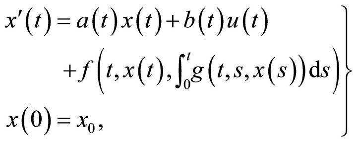
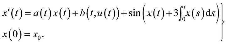
Consider the nonlinear scalar system
 (2.1)
(2.1)
for all . Here,
  is an
is an  function defined on
  and
and . For
. For , the state
  and the control
  belong to
 . Further,
  is a nonlinear function satisfying the Caratheadory conditions, i.e. f is measurable with respect to first argument and continuous with respect to second argument. Also,
  is a nonlinear function which also satisfies the Caratheadory conditions, where
 .
.
DEFINITION 2.1. The system (2.1) is said to be completely controllable on J if for any , and fixed T, there exists a control
  such that the corresponding solution
  of (2.1) satisfies
 .
.
It may be noted that according to the above definition, there is no constraint imposed on the control or on the trajectory.
REMARK 2.2. For the system (2.1), it is possible to steer any initial state  to any desired final state
 . But it does not give any idea about the path along which the system moves. Practically it may be desirable to steer the system from initial state
  to a final state
  along a prescribed trajectory. It may minimize certain cost involved in steering the system, depending upon the path chosen. It may also safe-guard the system. This motivates the study on the notion of T-controllability.
Let  be the set of all functions
  defined on
  such that
  and
and  is differentiable almost everywhere.
DEFINITION 2.3. The system (2.1) is said to be T-controllable if for any , there exists a control
  such that the corresponding solution
  of (2.1) satisfies
  a.e.
a.e.
DEFINITION 2.4. The system (2.1) is totally controllable on J if for all subintervals  of
of the system (2.1) is completely controllable.
Clearly, T-controllability  Total controllability
  Complete controllability.
In the system (2.1), both control  and state
  appear nonlinearly. First let us look at the following system where the control appears linearly.
 (2.2)
(2.2)
Assumptions [A1]
(i) The functions  and
and  are continuous on J.
(ii)  do not vanish on J.
(iii) f is Lipschitz continuous with respect to second and third argument, i.e. there exist  such that

for all 
(iv)  is
is  -Lipschitz continuous with respect to the third argument in the following sense.
Under the above assumptions, one can easily construct the control explicitly to prove the T-controllability of the nonlinear system (2.2). To see this we proceed as follows:
For each control , the existence and uniqueness of the solution for the system (2.2) follow from Assumptions [A1] by using the standard arguments.
Let  be a given trajectory in
 . We define a control function
  by
by
With this control, (2.2) becomes,
Setting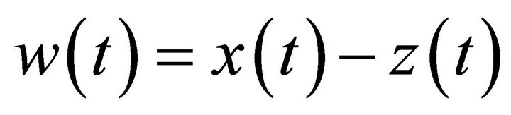 , we have
 (2.3)
(2.3)
By using the transition function  for the ordinary differential equation
 , (2.3) can be rewritten as
Thus
That is,
Hence by Grownwall’s inequality, it follows that
This proves T-controllability of the system (2.2).
As remarked earlier in the above nonlinear system (2.2), the control  is appearing linearly. Let us now consider the case in which control as well as the state appear nonlinearly as in (2.1). We have following theorem.
THEOREM 2.5. Suppose that
(i)  is continuous.
(ii)  is coercive in the second variable, i.e.
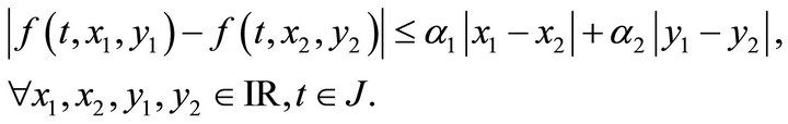
(iii) The function f is Lipschitz continuous in the second and third variable, uniformly in t, i.e. there exist  and
and  such that
(iv) The function g is Lipschitz in the third variable uniformly in , i.e., there exists
  such that

Then the nonlinear system (2.1) is T-controllable.
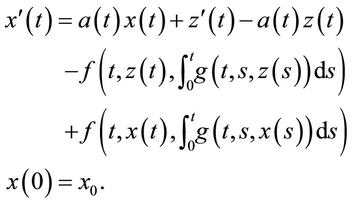
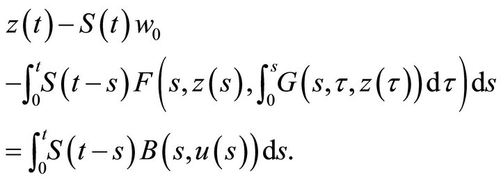
Proof: For each fixed u, the existence and uniqueness of the solution of the system (2.1) follow from the Lipschitz continuity of the functions f and g. Moreover, this solution satisfies the integral equation
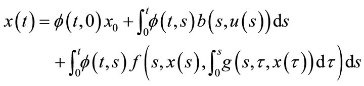 (2.4)
(2.4)
Let  be the prescribed trajectory with
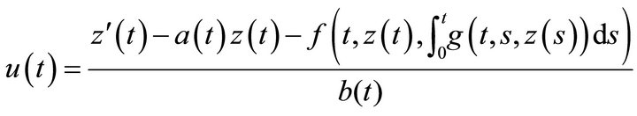
 . We want to find a control u satisfying
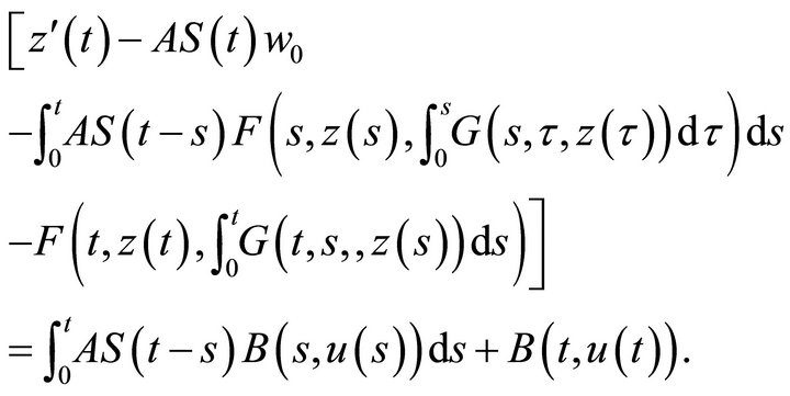
The above equation can be written as
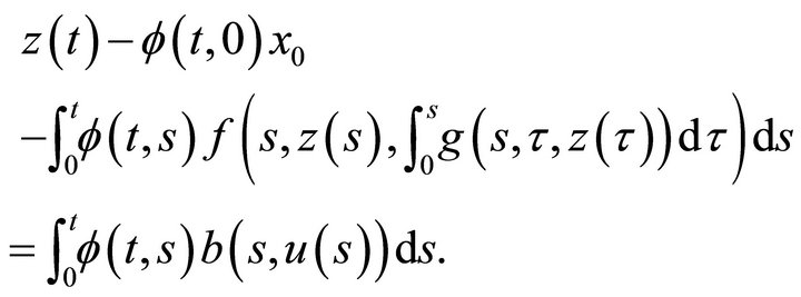
Differentiating with respect to t, we get
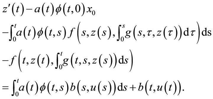 (2.5)
(2.5)
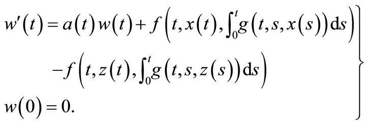
The Equation (2.5) can be written as
 (2.6)
(2.6)
where 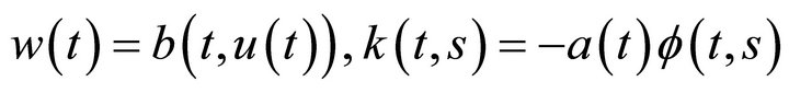 and
and
 is the left hand side of (2.5).
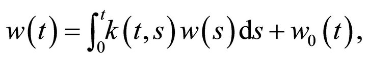
The Equation (2.6) is a linear Volterra integral equation of the second kind and it has a unique solution w(t) for each given  (refer [13]). Hence it suffices to extract
  from the solution
 . To extract
 , we use the technique of Deimling ( [14,15]).
Consider the multi-valued function  defined by
 . Since
and  are continuous, by hypothesis (ii)
  is nonempty for all t and upper semi-continuous. That is,
  implies
 . Further,
  has compact values. Hence
  is Lebesgue measurable and therefore has a measurable selection
 . This function u is the required control which steers the nonlinear system along the prescribed trajectory
 .
.
Hence proof is complete.
REMARK 2.6.
(i) The control u obtained in Theorem 2.5 is measurable, may not be continuous. But, if we require control u to be continuous, we have to assume more stronger condition on .
.
(ii) If the nonlinear function  is invertible then
  can be computed directly from
 . For example, if
  is strongly monotone i.e. there exists
  such that
then there exists a unique u such that . Note that the strong monotonicity implies coercivity.
(iii) If  is coercive and monotonically increasing with respect to u, then it can be seen that
  and
and  is solvable.
EXAMPLE 2.7. Consider the nonlinear integro-differential system with the control term 
The control term  is continuous and coercive. One can now verify f and g as in Theorem 2.5 to get T-controllability of the above system.
3. T-Controllability of Infinite-Dimensional Systems
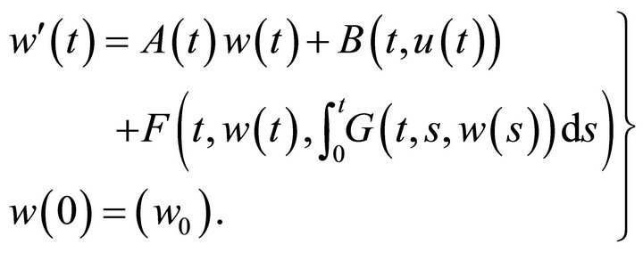
In this section we consider a nonlinear integro-differential system defined in infinite dimensional space and generalize the results of Section 2. Let H and U be Hilbert spaces and consider following nonlinear integrodifferential system.
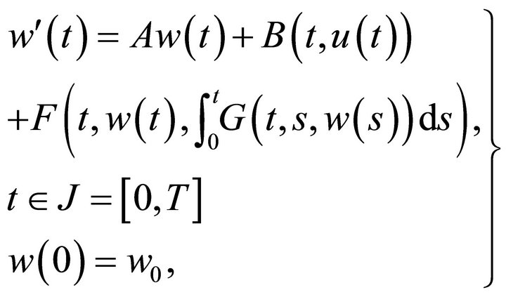 (3.1)
(3.1)
where the state  and the control
 , for each
 . The operator
  is a linear operator not necessarily bounded. The maps
 ,
,  and
and  are nonlinear operators, where
 .
.
We make the following assumptions on (3.1).
Assumptions [I]
(i) Let A be an infinitesimal generator of a strongly continuous  -semigroup of bounded linear operators
 . So there exist constants M1 ≥ 0 and
  such that
and also let
(ii) B and G satisfy Caratheadory conditions, i.e.  is continuous for
  and
and
 is measurable for
  and
and
 is continuous
  and
and
 is measurable
 .
.
(iii) F satisfies Caratheadory conditions like G.
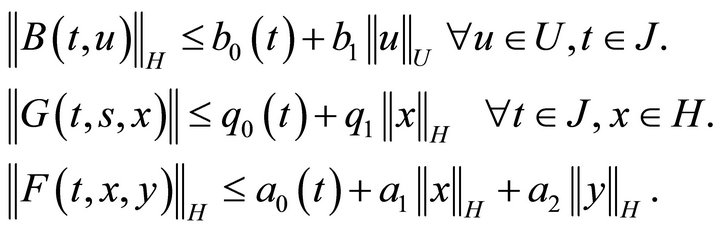
(iv)  satisfy following growth conditions
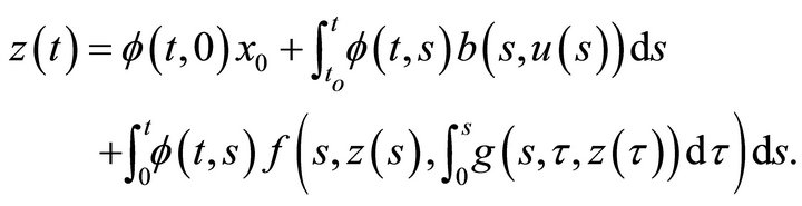
Under Assumptions [I], a mild solution of the system (1) satisfies the Volterra integral equation
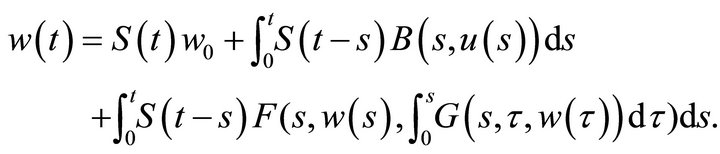 (3.2)
(3.2)
Let  be the set of all functions
  which are differentiable and
 . We say that the system (3.1) is T-controllable if for any
 , there exists an
  -function
  such that the corresponding solution
  of (1) satisfies
  a.e.
a.e.
We make the following additional assumptions on F and B.
Assumptions [II]
(i)  is Lipschitz continuous with respect to x and y, i.e. there exist constants
  such that

for all .
.
(ii)  is Lipschitz continuous with respect to
 , i.e. there exists a constant
  such that

(iii) B satisfies monotonicity and coercivity conditions, i.e.
and

We now prove the T-controllability result for the system (3.1).
THEOREM 3.1. Under Assumptions [I] and [II], the nonlinear system (3.1) is T-controllable.
Proof: Let z be any trajectory in . Following the proof of the Theorem 2.5, we look for a control u satisfying
Differentiating with respect to t, we get
 (3.3)
(3.3)
Equation (3.3) can be rewritten in the form
 (3.4)
(3.4)
where 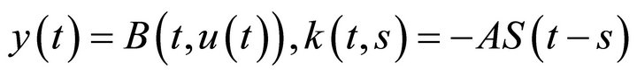 and
and  is the left hand side of (3.3).
Define an operator  by
by
 (3.5)
(3.5)
Assumption [I(i)] assures that K is a bounded linear operator [16]. Also, it can be easily proved that  is a contraction for sufficiently large n (refer [8,14]). Hence by generalized Banach contraction principle, there exists a unique solution y for (3.4) for given
 . Therefore, T-controllability follows if we can extract
  from the relation
 (3.6)
(3.6)
To see this, define an operator  by
by
 (3.7)
(3.7)
Assumptions [I(ii),(iii),(iv)] imply that N is welldefined, continuous and bounded operator. Assumption [II(iii)] shows that N is monotone and coercive. A hemicontinuous monotone mapping is of type  (see page 78 of [17]). Therefore, by Theorem 3.6.9 of Joshi and Bose [17], the nonlinear map N is onto. Hence there exists a control u satisfying (6). The measurability of
  follows as u is in
 . This proves Tcontrollability of the system (3.1).
COROLLARY 3.2. If F and G are Lipschitz continuous and B is strongly monotone, i.e. there exists  such that
 (3.8)
(3.8)
Then the system (3.1) is T-controllable.
Proof: The proof follows from the fact that the condition (3.8) implies Assumption [II(iii)].
REMARK 3.3. We have not directly used the Assumptions [II(i)] and [II(ii)] of the Lipschitz continuity of f in the proof of the Theorem 3.1. Actually, it is needed for the existence and uniqueness of the solution  satisfying (3.2) for each control
 . There are also other verifiable conditions for the uniqueness of the solution, in the literature (see [3]).
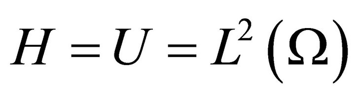
EXAMPLE 3.4. Let  be a bounded domain in
  with a smooth boundary
 . Consider the system
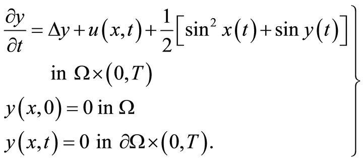
The above system can be put into the form of (3.1) by defining  for all
  where
where
 is the domain of A and
 . Here the control term
 is linear. The above system is T-controllable under the assumptions on F and G as in the theorem.
In the one dimensional case, say,  , one can explicitly write
 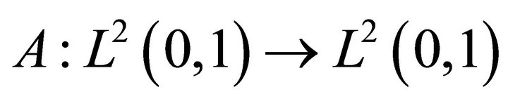 by
by , where
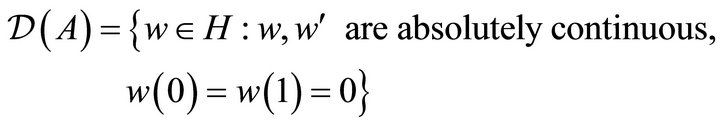
and
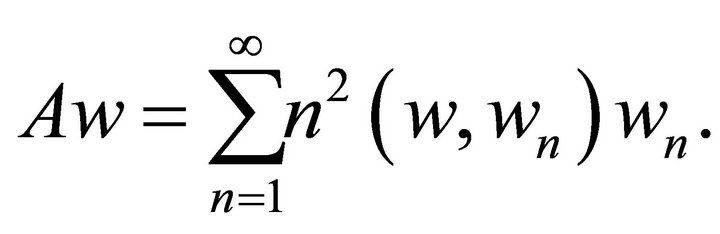
Here  is the orthogonal set of eigenfunctions of A and
  is the
  inner product. Further, A generates an analytic semigroup
  in H given by

Here 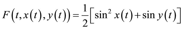 and
and , both are Lipschitz continuous.
We now specialize Theorem 3.1 for the case . So we consider the following finite dimensional nonlinear system in
 .
.
 (3.9)
(3.9)
where  are as in (3.1) with H replaced by
 . Therefore Theorem 3.1 can be specialized for the system (3.9) in
 . The following theorem can be proved as in Theorem 2.5.
THEOREM 3.5. Suppose that (i) F is Lipschitz continuous with respect to x and y and G is Lipschitz continuous in x (ii)  satisfies
Then the nonlinear system (3.9) is T-controllable by a measurable control 
EXAMPLE 3.6. Consider the nonlinear 2-dimensional system,
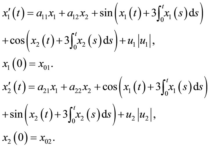
It can be easily verified that the above system satisfies the hypotheses of Theorem 2, and hence it is T-controllable.
4. Numerical Results
After discussing the T-controllability of various first order systems we will describe a method to numerically approximate the trajectory control and illustrate the results of these methods applied to Examples 2.7, 3.6 and 3.4. Generally, optimal control problems are posed to minimize some functional of the control function and state variables. Methods for numerically approximating these are well established. See [18-20] for descriptions of how to compute these approximations. As we do not have any functional of control or state to minimize, we will pose this problem as an optimization problem constrained by the state equations. Let the trajectory control  be defined by
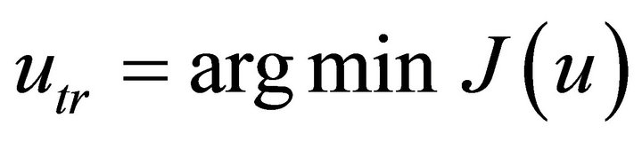
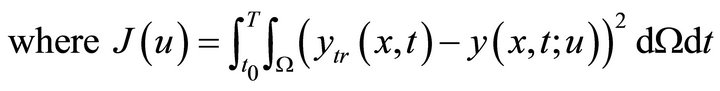
 (4.10)
where F defines the differential equations, y is the solution to that equation for a given u, and  is the desired trajectory. We will discretize the control in time,
 and space,
  , where k defines the spatial dimension (we will consider
 ),
),
 reducing the problem from the infinite dimensional problem of finding a
  to finding
 and interpolating for
  in between these points. To get an approximate solution to the differential equation for a given control we will discretize it using various finite difference techniques.
After we convert our trajectory control problem in Equation (4.10) into a discretized continous uncontrained optimization problem, we can solve it using various optimization rountines. We used two optimization routines in this work. The first method was a quasi-Newton algorithm with a finite difference gradient and a line search as implemented by the Matlab function fminunc.m. The second is a non-gradient method, Nelder-Mead, which attempts to minimize the function over a stencil of points that is varied by a series of rules to control the stencil size and shape, as implemented in the Matlab function fminsearch.m. Both algorithms are outlined in [21].
As this is a highly nonlinear optimization problem we will employ an interative type method of using these optimization routines. We attempted to use global type optimization routines with little success. The routine is as follows:
1) Pick an initial iterate defined over a coarse interval, i.e.  are small.
2) Use a gradient optimization routine to find an approximate trajectory control.
3) Use the control found from the gradient based method as the initial iterate for the non-gradient method, Nelder-Mead.
4) Increase  and find your new initial iterate by interpolating the old trajectory control over the now refined mesh.
5) Repeat steps 1 - 4 until the solution to your equation is satisfactorily close to your desired trajectory.
4.1. Integro Differential Equations
The first step in approximating the solution to Example 2.7 is to convert it to a higher order differential equation. Using the substitution  then the integro differential equations becomes the second order equation
 (4.11)
Making the substitutions  and
and  we can convert this second order equation into the following first order system of equations.
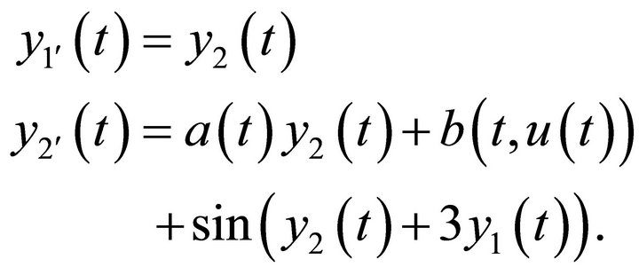 (4.12)
This sytem can then be solved using any general method for numerically approximating the solution to initial value problems. We used a variable order multistep solver implemented in Matlab’s ode15s.m. More details for this solver can be found in [22] and [23].
Figure 1 shows an example of the effects of optimization on finding the trajectory control. We simulated the differential equation on the interval  with a target of
 . We discretized the control and linearly interpolated the control values between the discretization points. We used the function
  and
and . Our intial control was
 . Our initial mesh was
  and we refined it to 10 and then 20 during the optimization. Our hybrid algorithm took 7.8 minutes on a PC running Windows 7, with an i5 processor and 4 GB of memory. All following simulations were run on the same machine. The final sum squared error between the state and the target was 0.0043, which results in an average absolute error of 0.02 per solution mesh point. Figure 1 illustrates how close the state gets to the target.
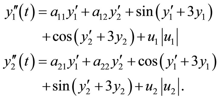
The system as shown in Example 3.6 was solved in a similar way. Making the substitution  and
and  you get the following system of second order ODEs
 (4.13)
Then using the substitutions ,
,  ,
,  ,
,  you get the following first order system of equations
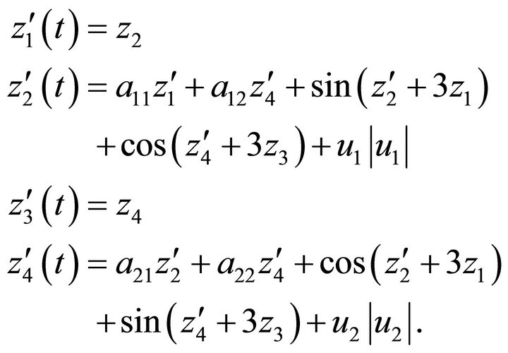 (4.14)
Again we sovle this using a variable order multistep solver implemented in Matlab’s ode15s.m.
We simulated the DE on the interval [0,10] with a targets of  and
and . We discretized each control with meshes of sizes n = 2, 4, 8, 16. This creates 4, 8, 16, and 32 total optimization points for controls
  and
and . We used the function
 . The optimization required 1 hour 25 minutes. The final sum squared error between the state and the target was 0.053, resulting in an average absolute error of 0.051 per discretization point. Figure 2 shows the results for the system of integro differential equations. Note how close the state gets to the target.
4.2. Partial Differential Equations
The nonlinear parabolic problem, as illustrated in Example 3.4 can be solved using built in Matlab software when working in only one spatial dimension. The function pdepe.m uses a second order spatial discretization to convert the PDE to a system of ODEs which can be solved using an implicit ODE solver [24].
The results for the target trajectory , with
 ,
,  and the PDE being discretized over a 20 by 20 grid can be seen in the following Figures 3 and 4. The initial interate for the control was
 , with intially
  which was then refined to
 . Our hybrid optimization method took 23.5 minutes. Note in Figure 3 how closely the solution to the PDE follows the desired trajectory. The optimal sum square error was
 . This results in a 0.0013 average absolute error for each of the 400 mesh points. Figure 4 illustrates how close this control methodology allows us to get to matching the desired trajectory at the end and the control function required to do it.
In two spatial dimensions there were no readily available software for this problem so we coded a finite difference scheme to approximate the solution. The spatial derivatives were approximated with a second order approximation as follows
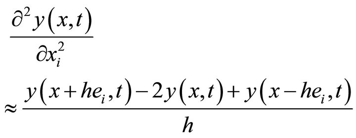 (4.15)
where h is defined by how finely the spatial mesh is defined and  is the canonical vector.
As parabolic equations are generally unstable for foward discretization schemes [25] and particularly for this problem we used backwards difference approximation for the time derivative,
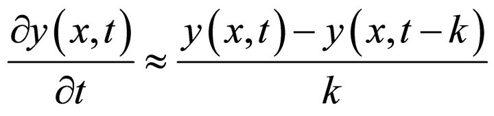 (4.16)
where k is determined by how finely the time variable is
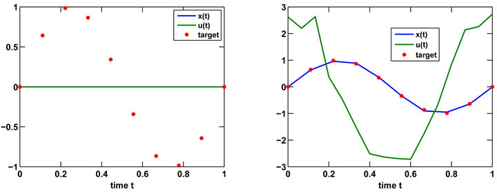
Figure 1. Numerical solution of the integro differential trajectory control problem. On the left is the state, control and target before optimization, i.e. with u(t) = 0. On the right are the state, control and target after optimization.
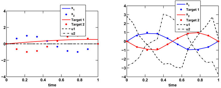
Figure 2. Numerical solution of the system of integro differential equations trajectory control problem. On the left is the state, control and target before optimization, i.e. u1(t) = u2(t) = 0. On the right are the state, control and target after optimization.
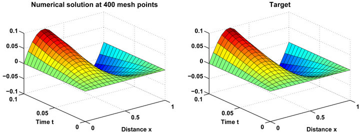
Figure 3. Numerical solution of first order PDE with desired trajectory on the right.
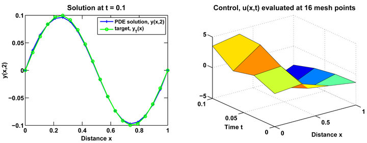
Figure 4. Numerical solution of first order PDE at t = 0.1 compared to the desired trajectory on the left. The trajectory control used to achived this result on the right.
discretized. This results in a backwards difference scheme for the solution to the PDE. The resulting system equations are not now explictily defined for future, in time, in terms of past values of . This results in a system of nonlinear equations for
  in terms of past approximations. We solve this nonlinear system of equations at each time step using a trust-region dogleg method [26] as implemented by the Matlab function fsolve.m.
The same general methodology was employed for the two spatial dimensional case, however the computational time was greatly increased and it is more difficult to visualize the control and the solutions. The results for the target trajectory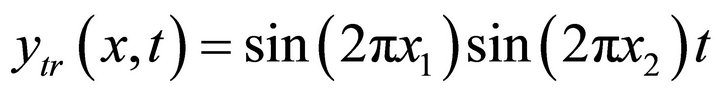 , with
 ,
,  were found with
 ,
,  and
and  creating a total of 64 points to optimize for and the PDE being discretized over a 20 by 20 grid can be seen in the following figures. Again a quasi-Newton method with a line search was used. Our iterative algorithm was tried but the addition of the nongradient method did not significantly improve results but did significantly increase computation time, so we do not include those results. First the optimization was performed only attempting to match the desired trajectory at
 . The computation took 15.1 hours. Then using this control as the initial iterate a second optimization was performed, with the original goal function where we attempt to match the trajectory over all of
 . This required 32.7 hours, resulting in a total of 47.8 hours for the total algorithm. The sum squared error over the 4000 mesh points was 0.1165. Giving an average absolute error of 0.0054 per mesh point. Note how close the PDE solution matches the desired trajectory as can be seen by in Figures 5 and 6.
5. Concluding Remarks
In this paper sufficient condotions for T-controllability of semilinear integro differential system in finite and infinite dimension spaces are proved by using measurable
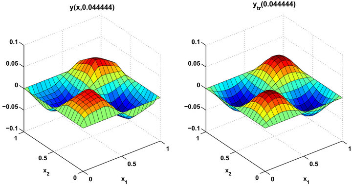
Figure 5. Numerical solution of PDE with control found through optimization at t = 0.4444.

Figure 6. Numerical solution of second order PDE with control found through optimization at t = 0.1.
selections, generalised Banach contraction principle and monotone operatory theory. Computational results for trajectory control required a wide variety of numerical techniques in two and three dimensions, including nonlinear optimization, equation solving and finite difference discretization. The numerical estimates justify the analytical proofs.
The method presented here is quite general and covers wide class of semilinear dynamical control systems. Similar results may be proved and computed for second order systems and semilinear dynamical control inclusions with delay arguments.
REFERENCES
- E. J. Davison and E. C. Kunze, “Controllability of Integro-Differential Systems in Banach Space,” SIAM Journal on Control and Optimization, Vol. 8, No. 1, 1970, pp. 489-497.
- R. K. George, “Approximate Controllability of Nonautonomous Semilinear Systems,” Nonlinear Analysis—TMA, Vol. 24, No. 1, 1995, pp. 1377-1393.
- R. K. George, D. N. Chalishajar and A. K. Nandakumaran, “Exact Controllability of Generalised Hammerstein Type Equations,” Electronic Journal of Differential Equation, Vol. 142, No. 1, 2006, pp. 1-15.
- J. L. Lions, “Exact Controllability, Stabilization and Perturbations for Distributed Systems,” SIAM Review, Vol. 30, No. 1, 1998, pp. 1-68. doi:10.1137/1030001
- D. N. Chalishajar, “Controllability of Nonlinear IntegroDifferential Third Order Dispersion Equation,” Journal of Mathematical Analysis and Applications, Vol. 348, No. 1, 2008, pp. 480-486. doi:10.1016/j.jmaa.2008.07.047
- R. K. George, D. N. Chalishajar and A. K. Nandakunaran, “Exact Controllability of Nonlinear Third Order Dispersion Equation,” Journal of Mathematical Analysis and Applications, Vol. 332, No. 2, 2007, pp. 1028-1044. doi:10.1016/j.jmaa.2006.10.084
- D. N. Chalishajar and F. S. Acharya, “Controllability of Neutral Impulsive Differential Inclusion with Nonlocal Conditions,” Applied Mathematics, Vol. 2, No. 1, 2011, pp. 1486-1496. doi:10.4236/am.2011.212211
- A. K. Nandakumaran and R. K. George, “Approximate Controllability of Nonautonomous Semilinear Systems,” Revista Mathematica UCM, Vol. 8, No. 1, 1995, pp. 181- 196.
- S. Micu and E. Zuazua, “On the Null Controllability of the Heat Equation in Unbounded Domains,” Bulletin des Sciences Mathématiques, Vol. 129, No. 2, 2005, pp. 175- 185. doi:10.1016/j.bulsci.2004.04.003
- F. Cardetti and M. Gordina, “A Note on Local Controllability on Li Groups,” System and Control Letters, Vol. 52, No. 12, 1990, pp. 979-987.
- J. Klamka, “Constrained Controllability of Semilinear Systems with Delayed Controls,” Bulletin of the Polish Academy of Sciences, Vol. 56, No. 4, 2008, pp. 333-337.
- J. Klamka, “Constrained Controllability of Semilinear Systems with Delay,” Nonlinear Dynamics, Vol. 56, No. 1-2, 2009, pp. 169-177. doi:10.1007/s11071-008-9389-4
- P. Linz, “A Survey of Methods for the Solution of Volterra Integral Equations of the First Kind in the Applications and Numerical Solution of Integral Equations,” Nonlinear Analysis—TMA, 1980, pp. 189-194.
- K. Deimling, “Nonlinear Volterra Integral Equations of the First Kind,” Nonlinear Analysis—TMA, Vol. 25, No. 1, 1995, pp. 951-957.
- K. Deimling, “Multivalued Differential Equations,” Walter De Gruyter, The Netherlands, 1992. doi:10.1515/9783110874228
- D. N. Chalishajar, “Controllability of Damped SecondOrder Initial Value Problem for a Class of Differential Inclusions with Nonlocal Conditions on Noncompact Intervals,” Nonlinear Functional Analysis and Applications (Korea), Vol. 14, No. 1, 2009, pp. 25-44.
- M. C. Joshi and R. K. Bose, “Some Topics in Nonlinear Functional Analysis,” Hasted Press, New York, 1985.
- M. D. Gunzburger, “Perspectives in Flow Control and Optimization. Advances in Design and Control,” SIAM: Society for Industrial and Applied Mathematics, Philadelphia, 2003.
- E. Polak, “Computational Methods in Optimization,” Academic Press, Cambridge, 1971.
- J. A. David, H. T. Tran and H. T. Banks, “HIV Model Analysis and Estimation Implementation under Optimal Control Based Treatment Strategies,” International Journal of Pure and Applied Mathematics, Vol. 57, No. 3, 2009, pp. 357-392.
- C. T. Kelley, “Iterative Methods for Optimization,” SIAM: Society for Industrial and Applied Mathematics, Philadelphia, 1999.
- L. F. Shampine and M. W. Reichelt, “The MATLAB ODE Suite,” SIAM Journal on Scientific Computing, Vol. 18, No. 1, 1997, pp. 1-22. doi:10.1137/S1064827594276424
- L. F. Reichelt, M. W. Shampine and J. A. Kierzenka. “Solving Index-1 DAEs in MATLAB and Simulink,” SIAM Review, Vol. 41, No. 3, 1999, pp. 538-552. doi:10.1137/S003614459933425X
- R. D. Skeel and M. Berzins, “A Method for the Spatial Discretization of Parabolic Equations in One Space Variable,” SIAM Journal on Scientific and Statistical Computing, Vol. 11, No. 1, 1990, pp. 1-32. doi:10.1137/0911001
- R. L. Burden and J. D. Faires, “Numberical Analysis,” Brookes/Cole Publisher, Salt Lake City, 2011.
- C. T. Kelley, “Iterative Methods for Linear and Nonlinear Equations,” SIAM: Society for Industrial and Applied Mathematics, Philadelphia, 1995. doi:10.1137/1.9781611970944
NOTES
*This paper is the extended version of http://math.iisc.ernet.in/ñands/2010-traj-DGNA_Franklin.pdf written by D. N. Chalishajar, R. K. George, A. K. Nandakumaran, F. S. Acharya, Journal of Franklin Institute, Vol. 347, 2010, pp. 1065-1075.
#Corresponding author.