Wireless Sensor Network, 2010, 2, 562-570
doi:10.4236/wsn.2010.27068 Published Online July 2010 (http://www.SciRP.org/journal/wsn)
Information-Driven Collaborative Processing for Diffusive
Source Estimation in Wireless Sensor Networks
Hossein Khonsari, Mohammad Hossein Kahaei
Electrical Engineering Department, Iran University of Science and Technology, Tehran, Iran
Received April 6, 2010; revised April 21, 2010; accepted May 2, 2010
Abstract
This paper discusses an accurate distributed algorithm for diffusive source localization while maintaining the
low energy consumption of sensor nodes in wireless sensor networks. In this algorithm, the sensor selection
scheme based on the information utility measure is used. To update the estimation in each selected node, a
neighborhood radius equal to the communication range of the sensor nodes is defined and all sensors located
in the neighborhood circle, whose radius is equal to the neighborhood radius and the selected node is its cen-
tre, collaborate their information. To decrease the energy consumption, the neighborhood radius is reduced
gradually based on the error covariance value of the estimation. In addition, this paper includes a new
method for the initial point calculation which is important in the recursive methods used for distributed algo-
rithms in wireless sensor networks. Numerical examples are used to study the performance of the algorithms.
Simulation results show the accuracy of the new algorithm becomes better while its energy consumption is
low enough.
Keywords: Information-Driven Collaborative Processing, Wireless Sensor Network, Diffusive Source
Localization
1. Introduction
Densely scattered low-cost sensor nodes provide a rich
and complex information source about the sensed world.
A major application of wireless sensor networks is to
perform monitoring tasks like localization and tracking
of one or more targets in their coverage field. In this pa-
per, we focus on the localization of a diffusive source.
The problem under consideration has application in the
fields of security, environmental and industrial monitor-
ing and pollution control [1]. Since in a typical wireless
sensor network each sensor node has limited battery
power, efficient collaborative signal processing algo-
rithms that consume less energy for computation and less
bandwidth for communication is needed [2]. In central-
ized estimation methods, sensor nodes transmit their row
observations to a fusion centre for processing [3-5]. How-
ever, some of their innate properties such as high-energy
consumption limit their use in a wireless sensor network
[6]. Therefore, recent research has concentrated on de-
veloping distributed processing.
Most of the current distributed estimation methods are
categorized in to two groups. In one group, the distrib-
uted estimation is developed using the sequential Bayes-
ian method [7-9]. In this method, the state belief (poste-
rior density function) is updated in the selected nodes
and when the quality of estimation is good enough (base
on the predefined threshold), the sensor selection is
stopped and the location is estimated. The most impor-
tant disadvantage of this type of method is that the con-
vergence of the estimation is not easy to be proven [6].
In the other group, the distributed estimation is yielded
by implementing the common centralized estimation
methods like Maximum Likelihood (ML) estimation in a
distributed manner [10]. As in this type the communica-
tion burden is high, the most important challenge is to
develop the accuracy of algorithms while considering the
total energy consumption. In this paper, we propose a
new method to improve the accuracy of diffusive source
estimation while maintaining the energy consumption in
a reasonable level.
The recent relevant work is presented in [6] where a
distributed Information-Driven Collaborative Processing
(IDCP) is derived. The essential point in this algorithm is
that by applying information utility measure, a sequence
of sensor nodes is chosen to reduce the required data
communications under the framework of ML estimation;

H. KHONSARI ET AL.
563
however, for estimation update, only selected node ob-
servations are used. In this paper, we propose the modi-
fication of the above method to improve the estimation
performance. In our algorithm called Modified IDCP
(MIDCP), each node calculates the new estimation of the
target location by averaging over the information of its
own observation and neighbors. However, the energy co-
nsumption increases because of large amount of trans-
mission. To mitigate this energy consumption we pro-
pose Energy Efficient MIDCP (EFMIDCP) in which the
neighborhood radius is decreased gradually based on the
estimation covariance value. In general, Iterative meth-
ods used in distributed algorithms may not yield the ML
estimate if the initial value is not selected carefully.
Therefore, we propose a new method to calculate initial
value for the iteration algorithms in our scenario.
This paper is organized as follows. In Section 2, we
present the physical and statistical models of the released
substance distribution. The IDCP algorithm is investiga-
ted in Section 3. In Section 4, we propose the MIDCP
and EFMIDCP algorithms. Section 5 includes a new
method to calculate initial estimation in all of these itera-
tive algorithms. In Section 6 the numerical examples are
used to demonstrate the performance of the proposed
methods. Conclusions are presented in Section 7.
2. Problem Formulation
2.1. Physical Model of a Difusive Source
Let

,ctr denote the substance concentration diffuse-
ion at a position

,
x
yr and time t. For a source-free
volume and space-invariant diffusivity, without biome-
dical reaction during the transport of biochemical agents,
the concentration of a diffusing substance follows the
well-known diffusion equation [5]:
22
2
22
ccc
kck
t
x
y


 



(1)
Where k is called the diffusivity in units of kg/m2s and
dependence on r and t is omitted to simplify the presen-
tation. It has been proved that in a rectangular parallele-
piped space and for certain types of initial and boundary
conditions, the solution of (1) is the product of the solu-
tions of the two single spatial-variable problems [5]. That
is,
 
,,,
xy
ct ctctrrr (2)
where

,
x
ctr is the solution of the diffusion equation
with single spatial-variable x:
 
2
2
,,
x
cxt cxt
k
tx


 (3)
with the similar definition for

,
y
cyt. We use the dis-
tribution equation which is derived in [5] for a continu-
ous point diffusive source (our desired source). The con-
centration of our source in a semi-infinite medium is
obtained using the following integral:
 

3
2
0
2
,
8
-
exp4
I
t
t
ct
kt
d
kt




















 


r
rr
(4)
where


00
,
x
y
0
r represents the exact source location,

is the substance realizing rate and
I
t is the initial
time of diffusion.
2.2. Statistical Measurement Model
We assume that a continuous point diffusive source is at
position 00 (, )
x
y

0
r, from which the diffusion sub-
stance is liberated continuously at a certain rate μ and at
time
I
t. The sensor nodes of a WSN are deployed in
which each sensor node is located at a known position
and can measure the substance concentration from the
diffusive sources. The measurement taking by sensor
node i at time
j
t can be written as:
2
(, )(, )(, )
(, )(0,),
ij ijij
ij
y
tctbet
er tN 
rr r
 (5)
where i
r is the known location of sensor node I, the
term (, )
ij
ctr is the concentration distribution shown in
Equation (4), b is a constant bias term representing the
sensor’s response to foreign substances assumed to be a
known and (, )
ij
etr is the sensor measurement’s Gaus-
sian noise independent in space and correlated in time,
i.e.,
 
12
112 2
12
12
,, .
0
jj
ijij
ii
etet ii










Er r (6)
Therefore, for each sensor node, we have ei

,1 ,
[ ,...,]T
iiN
ee, an N-dimension Gaussian distributed ran-
dom vector with the mean zero and covariance matrix
i

. By denoting(, )
iji j
yyt

r, (, )
iji j
eetr and
()( ,)
iji j
ct



θr, we can rewrite (1) as:
.
T
ij ijij
yea(θ)x (7)
Where () (),1
T
ij ij






aθθ
and


,
ij ij
crt  θ,

H. KHONSARI ET AL.
564
[,]
T
b  x is called the linear parameter vector and
00
[, ]
T
x
yθ represents the source parameters.
3. Information-Driven Collaborative
Processing
M sensor nodes are activated to estimate the location of
the diffusive source located in the network’s range. The
covariance matrix, i , is known for each node because
this matrix can be estimated during the calibration step in
practical applications. The measurements 

1,...,yy
M
of
all sensor nodes can be written as a vector form [6]:
y=A(θ)x + e (8)
where 1
yy,...,yT
TT
M


is a 1
M
N

vector, 1 () (),AθAθ
T


...,A(θ)T
T
M
 is aMN2matrix and 1,...,ee e
T
TT
M


repr-
esents the additive Gaussian noise. Regarding to the as-
sumptions, it follows a MN-dimension multiple normal
distribution with mean zero and covariance matrix Σ
with 

1,...,diag
M
ΣΣΣ
, Σ is diagonal because
the measurement noise of each two sensors is independ-
ent. We assume each sensor-node takes N samples.
According to the above measurement model, the log-
likelihood function of the measurements vector y is [6]:
1
1
1
()
1
=log2log
2
1
.
2
M
i
i
MT
ii iii
i
L
M
N
AA










y;θ
y(θ)xy (θ)x
(9)
By maximizing this log-likelihood function, the ML
estimation of θ is obtained:
1
1
ˆarg min
()().
MT
ii iii
i




 




θ
yAθxΣyAθx

(10)
To derive a distributed estimation, it is necessary to
use an incremental optimization method. Therefore, the
Gauss- Newton method is used to implement a distrib-
uted estimation. When employing this method to solve
the non-linear weighted least-square problem in (10), an
iterative process is obtained to update the estimate of θ
[6]:
(1) ()
1
() 1()
() 1()
()()
()(()),
kk
Tk k
kk
HH
HA
+
-
-
-
=
éù
+S
êú
ëû
´S-
θθ
θθ
θyθx
(11)
where
[]
()
() ,
A
H¶ =¶
θx
θ
θ
is an
M
NP´ Jacobian ma-
trix, when P parameters of desired source are unknown.
As it is necessary to collect all sensor node observations
to update the estimation, it is not a fully distributed algo-
rithm. So, the fully distributed information-driven col-
laborative processing (IDCP) investigated in the next
section.
3.1. Distributed Information_Driven Maximum
Likelihood Estimation
It is proven that the update stage of the Gauss-Newton
method can be divided in to a sequence of updates at
each sensor node. By applying this idea, instead of tran-
smitting the messages through all the sensor nodes, at
each sensor node some information is used to update the
estimation and determine which sensor in the neighbor of
the current node is the best one regarding information
amount (more details are in [6]).
The algorithm is initialized by sensor node i=1. It is
assumed that an initial value of θ is available at this
sensor node, denoted by(0)
ˆ
θ.
At sensor node i, the following steps are performed:
 Data receiving: the sensor node i has been acti-
vated by the previous node and has received the
transmitted required data.
 New variable calculation: Calculate the new ma-
trix (1)
ˆ
()
i
i

Hθ as
(1)
(1)
ˆ
()
ˆ
() ;
i
iAi
HiT







θθ
θx
θ
θ
(12)
then, update the information utility matrix, i
Γ, as
1
(1) 1(1)
ˆˆ
()().
ii
Ti i
iii
HH

 


θθ
(13)
 Estimation update: Update and obtain the current
estimate ˆi() θ as

()( 1)
1(1)1 (1)
ˆ
ˆ().
ii
Ti i
iiiii
HA

 




θ
θyx

 (14)
 Estimation quality test: Test the quality of the
updated parameter, ˆi()
θ, according to some per-
formance measures, e.g., the trace or determinant
of the covariance matrix in each sensor-node. If
the estimation of parameter is “good enough,”
the estimation process is terminated; otherwise,
the algorithm continues with the following steps.
 Sensor node selection: Select a sensor node from
its neighbor according to the certain information

H. KHONSARI ET AL.
565
utility criteria. The selected node should provide
the information that has the most potential to de-
crease the estimation uncertainty and increase the
performance.
In [6], the Cramer-Rao bound is chose as information
utility criteria and the estimation performance for two
reasons: 1)The CRB is the lower bound on the variance
of any unbiased estimators; it equals the inverse of the
Fisher information matrix (FIM). Hence, the measures
are calculated directly from the FIM. 2) The calculation
of the FIM as a performance measure is an intrinsic part
of the algorithm, i.e., it can be obtained without any extra
computation and data transmission. In [6] the recursive
equation for FIM is obtained. By denoting the matrix

i
Fθ in the sequence

 
,1,2,...
i
Fiθ as the FIM
of the parameter θ when collect the measurements
from the first i sensor nodes, i.e.,

1i
y=y,..., y, and
according to the definition of FIM [11,12],
 


2
2
1
ln y;
ln ;
=
iT
i
iT
p
FE
p
FE



 









θ
θ
θθ
yθ
θ
θθ
(15)
The second term on the Right Hand Side (RHS) of (16)
can be calculated as [6]:

 
 
2
1
ln ;
lny ;ln;
=
=
i
T
ii
T
T
iii
p
E
pp
E
HH














yθ
θθ
θyθ
θθ
θθ
(16)
Where
  
1
xx
....
ii
i
P
AA
H









θθ
θ
Hence, the recursive equation for the FIM sequence is
obtained as:
 


1
1
T
ii iii
FF HH


θθθθ (17)
By comparing (17) and (13) it can be easily observed
that the updating formulas for the matrix

i
Fθ and i

are the same. This equivalence represents that using FIM
as the performance measure will not increase the com-
putation complexity and the required transmission.
Consequently, if the trace of the FIM matrix is used as
the information measure, the information utility function
for node selecting is:

1
(;)( )( ).
T
lll
IlTr HH

θθθ (18)
Then, the sensor node l that maximizes this informa-
tion utility function is selected as the next sensor node
i+1:
1argmax(;)
lS
iIl


θ (19)
 Data transmission: The current sensor node trans-
mits the current estimate ˆi()
θ and i  to the se-
lected node and then the current node returns to
sleeping status.
4. Modified Information-driven
Collaborative Processing and
Energy Efficient Algorithms
4.1. Modified Information-Driven Collaborative
Processing
In wireless sensor networks, good collaboration among
distributed sensor nodes can be very useful to improve
estimation accuracy and keep the energy consumption in
a reasonable level. In the following, we propose a new
approach for estimation update motivated by the above
distributed estimation, i.e., IDCP. Here, we assume that S
is the collection of the sensor nodes located in the
neighbor area of the current sensor node i and lS

;


0
:,
li
Sl rrr (20)
Where i r, 0 r represent the location of the ith sensor
node and the neighborhood radius (here sensing range)
of the sensor nodes, respectively.
Through this approach, the sensor node i sends the
update information, (1)
ˆi

θ, to all of its neighbors, then
all these neighbors calculate the new private Jacobian
matrix, (1)
ˆ
()
i
l

Hθ, and information utility matrix, l Γ.
Based on these calculated matrixes, each node obtains
the ()
ˆl
θ as:


()-1( 1)
1(1)
ˆˆ
ˆ
().
iTi
lll
i
lll
H
A








θθ
Σyθx

(21)
Each node transmits ()
ˆi
i
θ to the ith node when this
node also performs the step 2 and 3 of IDCP algorithm to
obtain ()
ˆi
i
θ. Consequently, the estimation is updated as
follow:
()
1
1
()
ˆ.
i
l
L
l
i
L
 θθ
(22)
Note that in (22) the estimated value of current node,
()
ˆi
i
θ, is included because the current node is considered
in its neighborhood set. In our new algorithm, Modified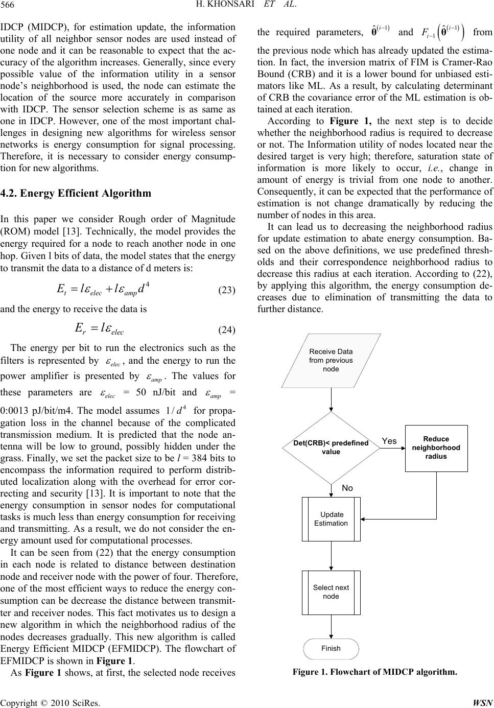

H. KHONSARI ET AL.
566
IDCP (MIDCP), for estimation update, the information
utility of all neighbor sensor nodes are used instead of
one node and it can be reasonable to expect that the ac-
curacy of the algorithm increases. Generally, since every
possible value of the information utility in a sensor
node’s neighborhood is used, the node can estimate the
location of the source more accurately in comparison
with IDCP. The sensor selection scheme is as same as
one in IDCP. However, one of the most important chal-
lenges in designing new algorithms for wireless sensor
networks is energy consumption for signal processing.
Therefore, it is necessary to consider energy consump-
tion for new algorithms.
4.2. Energy Efficient Algorithm
In this paper we consider Rough order of Magnitude
(ROM) model [13]. Technically, the model provides the
energy required for a node to reach another node in one
hop. Given l bits of data, the model states that the energy
to transmit the data to a distance of d meters is:
4
telecamp
E
lld   (23)
and the energy to receive the data is
relec
E
l

 (24)
The energy per bit to run the electronics such as the
filters is represented by elec

, and the energy to run the
power amplifier is presented by amp

. The values for
these parameters are elec

= 50 nJ/bit and amp

=
0:0013 pJ/bit/m4. The model assumes 4 1/ d for propa-
gation loss in the channel because of the complicated
transmission medium. It is predicted that the node an-
tenna will be low to ground, possibly hidden under the
grass. Finally, we set the packet size to be l = 384 bits to
encompass the information required to perform distrib-
uted localization along with the overhead for error cor-
recting and security [13]. It is important to note that the
energy consumption in sensor nodes for computational
tasks is much less than energy consumption for receiving
and transmitting. As a result, we do not consider the en-
ergy amount used for computational processes.
It can be seen from (22) that the energy consumption
in each node is related to distance between destination
node and receiver node with the power of four. Therefore,
one of the most efficient ways to reduce the energy con-
sumption can be decrease the distance between transmit-
ter and receiver nodes. This fact motivates us to design a
new algorithm in which the neighborhood radius of the
nodes decreases gradually. This new algorithm is called
Energy Efficient MIDCP (EFMIDCP). The flowchart of
EFMIDCP is shown in Figure 1.
As Figure 1 shows, at first, the selected node receives
the required parameters,

1
ˆi
θ and


1
1ˆi
i
F
θ from
the previous node which has already updated the estima-
tion. In fact, the inversion matrix of FIM is Cramer-Rao
Bound (CRB) and it is a lower bound for unbiased esti-
mators like ML. As a result, by calculating determinant
of CRB the covariance error of the ML estimation is ob-
tained at each iteration.
According to Figure 1, the next step is to decide
whether the neighborhood radius is required to decrease
or not. The Information utility of nodes located near the
desired target is very high; therefore, saturation state of
information is more likely to occur, i.e. , change in
amount of energy is trivial from one node to another.
Consequently, it can be expected that the performance of
estimation is not change dramatically by reducing the
number of nodes in this area.
It can lead us to decreasing the neighborhood radius
for update estimation to abate energy consumption. Ba-
sed on the above definitions, we use predefined thresh-
olds and their correspondence neighborhood radius to
decrease this radius at each iteration. According to (22),
by applying this algorithm, the energy consumption de-
creases due to elimination of transmitting the data to
further distance.
Receive Data
from previous
node
Det(CRB)< predefined
value
Update
Estimation
Select next
node
Reduce
neighborhood
radius
Finish
Yes
No
Figure 1. Flowchart of MIDCP algorithm.

H. KHONSARI ET AL.
567
5. New Method for Initial Target Location
Estimation
All iterative algorithms, such as Gauss-Newton method,
are sensitive to the initial point of estimation. For better
conception, a sample function for the estimation error is
shown in Figure 2. It can be seen that many sub-opti-
mum points exist in error function. Thus, if the initial
point is not estimated accurately, the algorithm requires
much iteration to diverge; even in some cases the diver-
gence is probable.
The method that we will propose in this section needs
at least three sensor nodes. As we mentioned before, the
distribution model for a diffusive source is:


0
00
,42 ct erf
kkt t








rr
rrr (25)
Where

2
0
2xt
erf xedt


 If the observation of
one node can satisfy


2
00
/4
i
tt krr, the erf
function is approximately one and with renunciation of
noise, the observation of this node is equal to:

0
,4
i
i
yb
k


 

rrr (26)
Therefore,
 

1
21
11
010
11
20 10
y, y,
y, y,
3
i
iin


 
 



rr
rr
rr rr
rr rr
(27)
y
x
-5
-10
-15
-20
56
-log [f(θ)]
54 52 50 48 46 44 44 46 48 50 52 54
Figure 2. Logarithm of the error function of a distributed
ML algorithm [14].
If n = 4, two unknown variable, 

000
,
x
yr, exist
and they are obtained by using numerical methods to
solve the set of equations and if n > 4 these are obtained
by solving set of equations and then averaging over the
results. In our proposed algorithm, we choose one node
arbitrary and this node is considered as the central proc-
essor. It gathers all observation of its neighbor nodes and
solves (27) to achieve the initial point for estimation. In
addition, this node is the first node in our sequence of
selected node.
6. Numerical Examples
This section presents a simulation of a sensor network
with M = 100 sensor nodes, distributed randomly in a
100?00mfield. At each sensor, the measurement of the
diffusive source is generated according to (5). Here,
source position 000
(, )
x
y

r is the unknown parameter
we need to estimate. We define a pair of neighbor sensor
nodes whose distance is less than 20m, i.e., the commu-
nication range (neighborhood radius) is 20 m. For the
diffusion model, we consider the environment as ho-
mogenous semi-infinite with an impermeable boundary
which can represent dispersion in air above the ground.
We use a scenario of a stationary impulse source located
at 0(50,30)

r meter. The bias term in (5) is 5 10b


g/m2, and the noise standard deviation is -6 610  
g/m2. We take 10 temporal samples at each sensor node
with a sampling interval of 5 seconds. The other pa-
rameters

, k, and
I
t are taken to be 1 g/s, 20 m2/s
and 0 s, respectively.
In Figure 3, the trajectory of target estimation for
IDCP and MIDCP is shown. The trajectory is depicted
with 10 iterations of both algorithms. This figure is the
result of averaging over 200 independent experiments in
which the location of sensor nodes and target are as-
sumed constant but the observations and measurement
noise of each sensor changes. In addition, the initial
value for estimation is obtained based on our proposed
algorithm in Section 5. In this figure, the “star” denotes
the exact location of the desired target and “triangles”
denote estimated location at each iteration. We observe
that although the initial bias is relatively high, the trajec-
tory nearly reach to the exact source location in MIDCP.
This means the algorithm can converge accurately and
nearly in comparison with IDCP.
For better conception, we compare bias estimation and
covariance error of these two algorithms in the following.
In Figures 4 and 5 we compare the estimation bias
2
ˆ

  of θ and the logarithm of determinant of
CRB for IDCP and MIDCP with respect to the number

H. KHONSARI ET AL.
568
of iterations. These figures are the result of averaging
over 200 independent experiments in which the location
of the sensor nodes and target are constant, but the ob-
servations and measurement noise of each sensor change.
10 203040 5060 70
10
20
30
40
50
60
70
X(m)
Y(m)
(a)
10 20 30 40 50 6070
10
20
30
40
50
60
70
X(m)
Y(m)
(b)
Figure 3. Trajectory of target estimation in a square area
with 100 sensor nodes randomly placed for a) IDCP and b)
MIDCP.
05 10 15 2025 30 3540
0
2
4
6
8
10
12
Numbr of Iteation
Estimation Bias(m)
IDCP
MIDCP
Figure 4. Estimation bias versus number of iterations for
IDCP and MIDCP algorithms.
According to these two above figures, we find that the
estimation performance of MIDCP is much better than
IDCP and this means that using all information utilities
of neighbor sensors can greatly improve the accuracy of
the estimation.
Before we discuss the simulation results for EF-
MIDCP, we provide the estimation bias and energy con-
sumption of MIDCP with the different neighborhood
radiuses. At first, we calculate the energy consumption
for neighborhood radiuses equal to 5, 10, 15, 20 for
MIDCP based on (23) and (24). The experiment condi-
tions are similar to the previous one. The results are
shown in Table 1.
As can be seen, by increasing the neighborhood radius
(communication range) the energy consumption increase
and the bias estimation decreases. Therefore, it is a
tradeoff between the accuracy of the algorithm and the
bias estimation. It motivates us to decrease the energy
consumption without dramatic change in the accuracy of
the algorithm; we decrease the neighborhood range with
regard to the error covariance of MIDCP calculated at
each iteration. (See Section 4.)
In the second example, we compare the performance
of MIDCP with EFMIDCP. In Figures 6 and 7 the esti-
mation bias
2
ˆ

 of θand logarithm of determi-
nant of CRB with respect to the number of iterations are
shown. These figures are the result of averaging over 200
independent experiments in which the location of sensor
Log determinant of CRB
05 10 15 20 25 30 35 40
-6
-5.5
-5
-4.5
-4
-3.5
-3
Number of Iterations
IDCP
MIDCP
Figure 5. Log determinant of CRB versus number of itera-
tions for IDCP and MIDCP algorithms.
Table 1. Energy consumption and estimation bias for MI-
DCP with different neighborhood radiuses.
20 15 10 5 Neighborhood radius
0.67 0.88 0.85 5.25 Bias Estimation(m)
24.38 4.9 1.56 0.14
Energy Used )μJ(

H. KHONSARI ET AL.
569
nodes and the target are assumed constant but the obser-
vations and measurement noise of each sensor change.
Other conditions are as same as our first example. In this
scenario, we change the neighborhood radius with the
following pattern:
 If log()4.5CRB  then the neighborhood ra-
dius is set to 20.
 If 5 log()4.5CRB then the neighborhood
radius is set to 15.
 If log() 5CRB  then the neighborhood radius
is set to 10.
According to these two figures, we find that the esti-
mation performance of MIDCP is somewhat better than
EFMIDCP. In addition, in this example we compare en-
ergy consumption of these tow algorithms and the result
is shown in Table 2. As it shows, the energy consump-
tion decreases dramatically and it can be observed that
the EFMIDCP reduces the energy consumption by half
while duplicates the accuracy of the algorithm.
05 10 15 20 25 30 35 40
0
2
4
6
8
10
12
Number Of Iterations
Estimation Bias(m)
EFMIDCP
MIDCP
Figure 6. Estimation bias versus number of iterations for
MIDCP and EFIDCP algorithms.
05 10 15 20 25 30 35 40
-6
-5.5
-5
-4.5
-4
-3.5
-3
Number of Iterations
Log Determinan CRB
EFMIDCP
MIDCP
Figure 7. Log determinant of CRB versus number of itera-
tions for MIDCP and EFMIDCP algorithms.
Table2. The energy and bias estimation for MIDCP and
EFMIDCP.
EFMIDCP MIDCP
1.45 0.67 Bias Estimation (m)
13.05 24.38
Energy Used )μJ(
7. Conclusions
In this paper, we addressed the problem of developing an
accurate and energy efficient distributed algorithm for a
diffusive source location estimation in wireless sensor
networks. At first, we defined the neighborhood radius
that was equal to the communication range of the sensor
nodes. Then, we used the information of every node loc-
ated within the neighborhood circle. This method im-
proved the accuracy of estimation. However, based on
ROM model, we observed that the energy consumption
in our new algorithm was somewhat high. As our pri-
mate goal was to reduce energy consumption and inc-
rease the accuracy, we proposed another algorithm in
which the neighborhood range decreased gradually based
on the covariance error of the estimation. In addition, we
proposed a new algorithm for the initial point calculation
which was necessary for iterative methods like Gauss-
Newton method. Finally, we used numerical examples to
compare the performance of our proposed methods and
found that EFMIDCP was the most suitable algorithm to
apply in wireless sensor networks when we considered
both energy consumption and the accuracy of the estima-
tion. In future work, a mathematical relationship between
the neighborhood radius and the number of covariance
error can be derived; therefore the neighborhood radius
can be changed adaptively instead of changing it with
regard to predefined value. In addition, the distributed
implementation of other recursive methods such as New-
ton method can be derived.
8. Acknowledgements
This research has been supported by Iran Telecommuni-
cation Research Center, Tehran, Iran, which is appreci-
ated.
5. References
[1] T. Zhao and A. Nehorai, “Detecting and Estimating Bio-
chemical Dispersion of a Moving Source in a Semi-Infi-
nite Medium,” IEEE Transactions on Signal Processing,
Vol. 54, No. 6, June 2006, pp. 2213-2225.
[2] X. Sheng and Y. H. Hu, “Maximum Likelihood Multiple-
Source Localization Using Acoustic Energy Measure-
ments with Wireless Sensor Networks,” IEEE Transac-

H. KHONSARI ET AL.
570
tions on Signal Processing, Vol. 53, No. 1, January 2005,
pp. 44-53.
[3] A. Pardo, S. Marco and J. Samitier, “Nonlinear Inverse
Dynamic Models of Gas Sensing Systems Based on
Chemical Sensor Arrays for Quantitative Measurements,”
IEEE Transactions on Instrumentation and Measurement,
Vol. 47, No. 3, June 1998, pp. 644-651.
[4] H. Ishida, T. Nakamoto and T. Moriizumi, “Remote sen-
sing and localization of gas/odor source and distribution
using mobile sensing system,” Proceedings of the Inter-
national Conference on Solid-State Sensors and Actua-
tors, Chicago, Vol. 1, June 1997, pp. 16-19.
[5] A. Nehorai, B. Porat and E. Paldi, “Detection and Locali-
zation of Vaporemitting Sources,” IEEE Transactions on
Signal Processing, Vol. 43, No. 1, January 1995, pp. 243-
253.
[6] T. Zhao and A. Nehorai, “Information-Driven Distributed
Maximum Likelihood Estimation Based on Gauss-New-
ton Method in Wireless Sensor Networks,” IEEE Trans-
actions on Signal Processing, Vol. 55, No. 9, September
2007, pp. 4669-4682.
[7] A. T. Ihler, J. W. Fisher, R. L. Moses and A. S. Willsky,
“Nonparametric Belief Propagation for Self-Localization
of Sensor Networks,” IEEE Journal on Selected Areas in
Communications, Vol. 23, No. 4, April 2005, pp. 809-
819.
[8] J. L. Williams, J. W. Fisher and A. S. Willsky, “Optimi-
zation Approaches to Dynamic Routing of Measurements
and Models in a Sensor Network Object Tracking Prob-
lem,” IEEE International Conference on Acoustics,
Speech, and Signal Processing (ICASSP), Philadelphia,
Vol. 5, March 2005, pp. 1061-1064.
[9] J. Liu, J. Reich and F. Zhao, “Collaborative In-Network
Processing for Target Tracking,” EURASIP Journal on
Applied Signal Processing, Vol. 2003, No. 4, 2003, pp.
378-391.
[10] M. G. Rabbat and R. D. Nowak, “Decentralized Source
Localization and Tracking,” IEEE International Confer-
ence on Acoustics, Speech, and Signal Processing
(ICASSP), Montreal, May 2004, pp. 921-924.
[11] P. Stoica and A. Nehorai, “MUSIC, Maximum Likeli-
hood, and Cramer-Rao Bound,” IEEE Transactions on
Acoustics Speech and Signal Processing, Vol. 37, No. 5,
1989, pp. 720-741.
[12] S. F. Yau and Y. Bresler, “A Compact Cramer-Rao
Bound Expression for Parametric Estimation of Super-
imposed Signals,” IEEE Transactions on Signal Proc-
essing, Vol. 40, No. 5, 1992, pp. 1226-1230.
[13] L. Kaplan, “Global Node Selection for Localization in a
Distributed Sensor Network,” IEEE Transactions on
Aerospace and Electronic Systems, Vol. 42, No. 1, Janu-
ary 2006, pp. 113-135.
[14] D. Blatt and A. O. Hero, “Energy-Based Sensor Network
Source Localization via Projection onto Convex Sets,”
IEEE Transactions on Signal Processing, Vol. 54, No. 9,
September 2006, pp. 3614-3619.