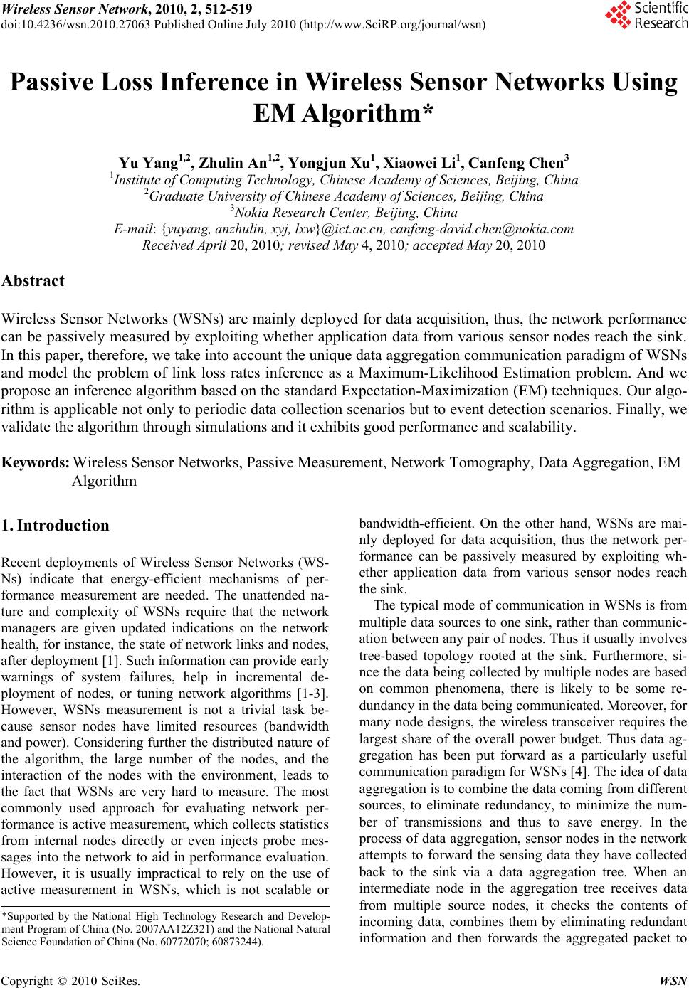Wireless Sensor Network, 2010, 2, 512-519
doi:10.4236/wsn.2010.27063 Published Online July 2010 (http://www.SciRP.org/journal/wsn)
Passive Loss Inference in Wireless Sensor Networks Using
EM Algorithm*
Yu Yang1,2, Zhulin An1,2, Yongjun Xu1, Xiaowei Li1, Canfeng Chen3
1Institute of Computing Technology, Chinese Academy of Sciences, Beijing, China
2Graduate University of Chinese Academy of Sciences, Beijing, China
3Nokia Research Center, Beijing, China
Received April 20, 2010; revised May 4, 2010; accepted May 20, 2010
Abstract
Wireless Sensor Networks (WSNs) are mainly deployed for data acquisition, thus, the network performance
can be passively measured by exploiting whether application data from various sensor nodes reach the sink.
In this paper, therefore, we take into account the unique data aggregation communication paradigm of WSNs
and model the problem of link loss rates inference as a Maximum-Likelihood Estimation problem. And we
propose an inference algorithm based on the standard Expectation-Maximization (EM) techniques. Our algo-
rithm is applicable not only to periodic data collection scenarios but to event detection scenarios. Finally, we
validate the algorithm through simulations and it exhibits good performance and scalability.
Keywords: Wireless Sensor Networks, Passive Measurement, Network Tomography, Data Aggregation, EM
Algorithm
1. Introduction
Recent deployments of Wireless Sensor Networks (WS-
Ns) indicate that energy-efficient mechanisms of per-
formance measurement are needed. The unattended na-
ture and complexity of WSNs require that the network
managers are given updated indications on the network
health, for instance, the state of network links and nodes,
after deployment [1]. Such information can provide early
warnings of system failures, help in incremental de-
ployment of nodes, or tuning network algorithms [1-3].
However, WSNs measurement is not a trivial task be-
cause sensor nodes have limited resources (bandwidth
and power). Considering further the distributed nature of
the algorithm, the large number of the nodes, and the
interaction of the nodes with the environment, leads to
the fact that WSNs are very hard to measure. The most
commonly used approach for evaluating network per-
formance is active measurement, which collects statistics
from internal nodes directly or even injects probe mes-
sages into the network to aid in performance evaluation.
However, it is usually impractical to rely on the use of
active measurement in WSNs, which is not scalable or
bandwidth-efficient. On the other hand, WSNs are mai-
nly deployed for data acquisition, thus the network per-
formance can be passively measured by exploiting wh-
ether application data from various sensor nodes reach
the sink.
The typical mode of communication in WSNs is from
multiple data sources to one sink, rather than communic-
ation between any pair of nodes. Thus it usually involves
tree-based topology rooted at the sink. Furthermore, si-
nce the data being collected by multiple nodes are based
on common phenomena, there is likely to be some re-
dundancy in the data being communicated. Moreover, for
many node designs, the wireless transceiver requires the
largest share of the overall power budget. Thus data ag-
gregation has been put forward as a particularly useful
communication paradigm for WSNs [4]. The idea of data
aggregation is to combine the data coming from different
sources, to eliminate redundancy, to minimize the num-
ber of transmissions and thus to save energy. In the
process of data aggregation, sensor nodes in the network
attempts to forward the sensing data they have collected
back to the sink via a data aggregation tree. When an
intermediate node in the aggregation tree receives data
from multiple source nodes, it checks the contents of
incoming data, combines them by eliminating redundant
information and then forwards the aggregated packet to
*Supported by the National High Technology Research and Develop-
ment Program of China (No. 2007AA12Z321) and the National Natural
Science Foundation of China (No. 60772070; 60873244).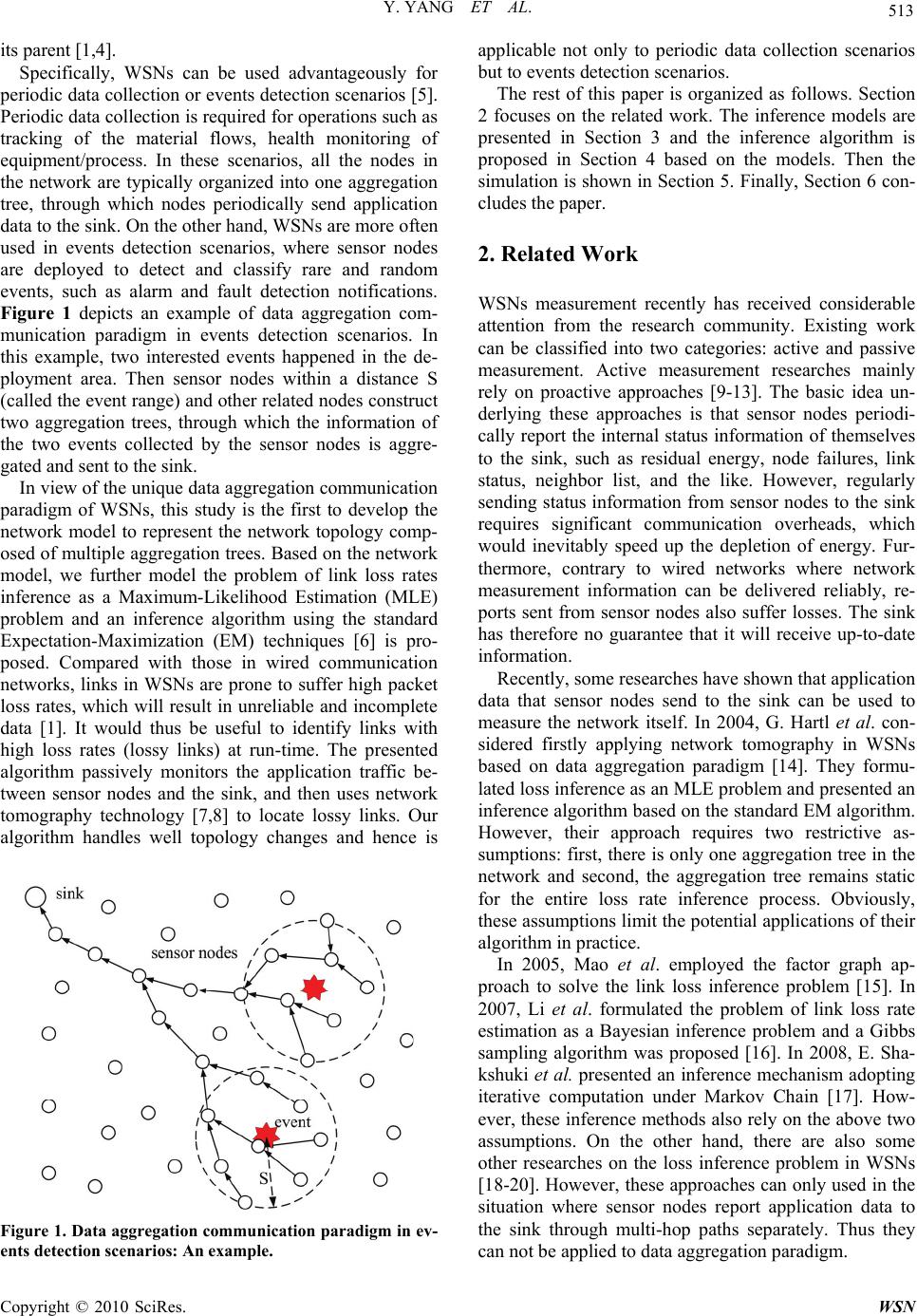

Y. YANG ET AL.
513
its parent [1,4].
Specifically, WSNs can be used advantageously for
periodic data collection or events detection scenarios [5].
Periodic data collection is required for operations such as
tracking of the material flows, health monitoring of
equipment/process. In these scenarios, all the nodes in
the network are typically organized into one aggregation
tree, through which nodes periodically send application
data to the sink. On the other hand, WSNs are more often
used in events detection scenarios, where sensor nodes
are deployed to detect and classify rare and random
events, such as alarm and fault detection notifications.
Figure 1 depicts an example of data aggregation com-
munication paradigm in events detection scenarios. In
this example, two interested events happened in the de-
ployment area. Then sensor nodes within a distance S
(called the event range) and other related nodes construct
two aggregation trees, through which the information of
the two events collected by the sensor nodes is aggre-
gated and sent to the sink.
In view of the unique data aggregation communication
paradigm of WSNs, this study is the first to develop the
network model to represent the network topology comp-
osed of multiple aggregation trees. Based on the network
model, we further model the problem of link loss rates
inference as a Maximum-Likelihood Estimation (MLE)
problem and an inference algorithm using the standard
Expectation-Maximization (EM) techniques [6] is pro-
posed. Compared with those in wired communication
networks, links in WSNs are prone to suffer high packet
loss rates, which will result in unreliable and incomplete
data [1]. It would thus be useful to identify links with
high loss rates (lossy links) at run-time. The presented
algorithm passively monitors the application traffic be-
tween sensor nodes and the sink, and then uses network
tomography technology [7,8] to locate lossy links. Our
algorithm handles well topology changes and hence is
Figure 1. Data aggregation communication paradigm in ev-
ents detection scenarios: An example.
applicable not only to periodic data collection scenarios
but to events detection scenarios.
The rest of this paper is organized as follows. Section
2 focuses on the related work. The inference models are
presented in Section 3 and the inference algorithm is
proposed in Section 4 based on the models. Then the
simulation is shown in Section 5. Finally, Section 6 con-
cludes the paper.
2. Related Work
WSNs measurement recently has received considerable
attention from the research community. Existing work
can be classified into two categories: active and passive
measurement. Active measurement researches mainly
rely on proactive approaches [9-13]. The basic idea un-
derlying these approaches is that sensor nodes periodi-
cally report the internal status information of themselves
to the sink, such as residual energy, node failures, link
status, neighbor list, and the like. However, regularly
sending status information from sensor nodes to the sink
requires significant communication overheads, which
would inevitably speed up the depletion of energy. Fur-
thermore, contrary to wired networks where network
measurement information can be delivered reliably, re-
ports sent from sensor nodes also suffer losses. The sink
has therefore no guarantee that it will receive up-to-date
information.
Recently, some researches have shown that application
data that sensor nodes send to the sink can be used to
measure the network itself. In 2004, G. Hartl et al. con-
sidered firstly applying network tomography in WSNs
based on data aggregation paradigm [14]. They formu-
lated loss inference as an MLE problem and presented an
inference algorithm based on the standard EM algorithm.
However, their approach requires two restrictive as-
sumptions: first, there is only one aggregation tree in the
network and second, the aggregation tree remains static
for the entire loss rate inference process. Obviously,
these assumptions limit the potential applications of their
algorithm in practice.
In 2005, Mao et al. employed the factor graph ap-
proach to solve the link loss inference problem [15]. In
2007, Li et al. formulated the problem of link loss rate
estimation as a Bayesian inference problem and a Gibbs
sampling algorithm was proposed [16]. In 2008, E. Sha-
kshuki et al. presented an inference mechanism adopting
iterative computation under Markov Chain [17]. How-
ever, these inference methods also rely on the above two
assumptions. On the other hand, there are also some
other researches on the loss inference problem in WSNs
[18-20]. However, these approaches can only used in the
situation where sensor nodes report application data to
the sink through multi-hop paths separately. Thus they
can not be applied to data aggregation paradigm.

Y. YANG ET AL.
514
3. Inference Models
In this section, we develop the models which are the ba-
sis for the inference. We first model the network and
then formulate the loss performance.
3.1. Network Model
Let N = (V(N), L(N)) denote a network with sets of nodes
V(N) and the set of links L(N). The sink is denoted by s
and is assumed to have greater resources available than
the other nodes. (i, j)  L(N) denotes a directed link from
node i to node j in the network. Let  denote a set of
aggregation trees embedded in N, i.e., T  , V(T) 
V(N) and L(T)  L(N). Note that (i, j) can appear in more
than one tree. Thus for (i, j)  L(N), we denote i,j  
the set of trees which include link (i, j). Let (q  p)T
denote the path from node q to node p in T and L((q 
p)T) denote the set of links on the path. The set of chil-
dren of node i in T is denoted by d(i, T) = {k  V(T) | (k,
i)  L(T)}. Define the set of leaf nodes in T by R(T), i.e.,
R(T) = {k  V(T) | d(k, T) = }. For k  V(T)\R(T), let
T(k) denote the subtree within T rooted at k. Then R(k, T)
= R(T) ∩ V(T(k)) is defined as the set of leaf nodes which
are descended from k in T. Also, we denote the set of all
of the leaf nodes in the network by ()
T
RRT

.
3.2. Loss Model
For each link an independent Bernoulli loss process is
assumed, which is a reasonable assumption [21]. Thus
(i, j)  L(N) can be associated with a transmission rate

i,j  (0,1). Let

i,j be the probability that packets sent
from node i to node j are received successfully by j. Ac-
cordingly, the loss rate of (i, j) is ,, 1

 
ij ij. The flow
of the data through an aggregation tree T therefore can be
modeled by a stochastic process XT = (Xp,q,T)p,qV(T),
where Xp,q,T  {0,1}. Xp,q,T = 1 means that the data sent
from node q were successfully received by intermediate
node p in the path (q  s)T. Similarly, Xp,q,T =0 means
that the data sent from q did not successfully reach p. Let
 = ( 
i,j)(i,j)L(N) denote the set of transmission rates for
all links.
We assume that information about which leaf nodes’
data is present in the aggregated data must also be bun-
dled into the aggregated packet. Thus for T  , con-
sider the collection of data by the sink to be an experi-
ment. Each round of data collection will be considered a
trial within this experiment. Suppose each leaf node tries
to send data in each round. The outcome of each trial
will be a record of which leaf nodes the sink received
data from in that round. It is worth noting that the infer-
ence method in [14] needs the record about all nodes in
the network, including leaf nodes and intermediate nodes.
Therefore our method is more practical than that in [14].
In terms of the stochastic process XT defined above,
each trial outcome is a random value XR(T) = (Xs,k,T) kR(T)
 ΩR(T) = {0,1}|R(T)|. Thus the overall outcome of  can
be denoted by () 
R
TRT
XX
. Let ΩR(T)(i) be the set of
outcomes XR(T) in which there is at least one node in R(i,T)
whose data were successfully received by the sink, i.e.,


()()()(,) ,,
(): 1.
RTRTRTk RiTskT
ix X


  (1)
Let nT denote the data collection rounds of T. The
probability of the nT independent observations of XR(T) is
then
() ()
1
(;)(;)
T
nm
RT RT
m
pX px



 (2)
and the probability of the observations of XR is
()
(;)(;).
RRT
T
pX pX





(3)
p(XR;  ) is the likelihood function, that is, the probabil-
ity that we observe the data XR given the link transmis-
sion rates
 . Therefore the problem of inferring link loss
rates from measurements at the sink can be formulated as
an MLE problem. That is, our goal is to estimate  by
ˆ

such that ˆ

maximizes the likelihood of observing
the outcomes of XR, i.e.,
ˆarg max(;).
R
pX




(4)
However, XR is not sufficient to obtain a direct expres-
sion for p(XR;  ) and then the above equation can not be
solved directly. Fortunately, the standard EM techniques
can be applied to the data taken from all of the trees to
efficiently solve the problem. The basic idea is that
rather than performing a complicated maximization, we
“augment” the observable data with unobservable data so
that the resulting likelihood has a simpler form.
4. Inference Algorithm
In this section, we further formulate the loss inference
problem as an MLE problem with complete observations
and then efficiently solve it using the EM algorithm. We
begin by presenting some brief background information
and then apply the EM algorithm to the loss inference.
4.1. Background
The EM Algorithm is a general method for finding MLE
of parameters in statistical models, where the model de-
pends on missing data [6]. Although a problem at first
sight may not appear to be an incomplete-data one (as it
is in our case), there may be much to be gained computa-
tion-wise by artificially formulating it as such to facili-
tate MLE. For many statistical problems, the complete-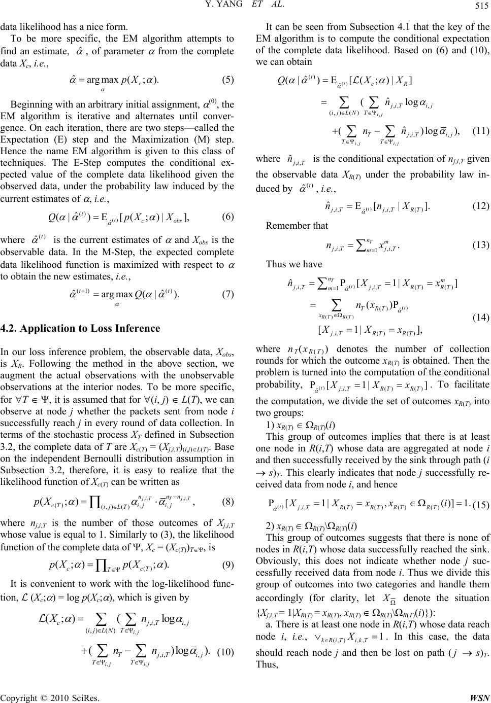

Y. YANG ET AL.
515
data likelihood has a nice form.
To be more specific, the EM algorithm attempts to
find an estimate, ˆ

, of parameter  from the complete
data Xc, i.e.,
ˆarg max(;).
c
pX


  (5)
Beginning with an arbitrary initial assignment, 
(0), the
EM algorithm is iterative and alternates until conver-
gence. On each iteration, there are two steps—called the
Expectation (E) step and the Maximization (M) step.
Hence the name EM algorithm is given to this class of
techniques. The E-Step computes the conditional ex-
pected value of the complete data likelihood given the
observed data, under the probability law induced by the
current estimates of
 , i.e.,
()
()
ˆ
ˆ
(|) E[(;)|],
t
t
c obs
QpXX

   (6)
where ()
ˆ

t is the current estimates of
 and Xobs is the
observable data. In the M-Step, the expected complete
data likelihood function is maximized with respect to 
to obtain the new estimates, i.e.,
(1) ()
ˆˆ
arg max(|).
tt
Q


 (7)
4.2. Application to Loss Inference
In our loss inference problem, the observable data, Xobs,
is XR. Following the method in the above section, we
augment the actual observations with the unobservable
observations at the interior nodes. To be more specific,
for T  , it is assumed that for (i, j)  L(T), we can
observe at node j whether the packets sent from node i
successfully reach j in every round of data collection. In
terms of the stochastic process XT defined in Subsection
3.2, the complete data of T are Xc(T) = (Xj,i,T)(i,j)L(T). Base
on the independent Bernoulli distribution assumption in
Subsection 3.2, therefore, it is easy to realize that the
likelihood function of Xc(T) can be written as
,, ,,
(), ,
(, )( )
(;),
jiTT jiT
nnn
cTij ij
ij LT
pX 



 (8)
where nj,i,T is the number of those outcomes of Xj,i,T
whose value is equal to 1. Similarly to (3), the likelihood
function of the complete data of , Xc = (Xc(T))T, is
()
(;)( ;).
ccT
T
pX pX



 (9)
It is convenient to work with the log-likelihood func-
tion,  (Xc;  ) = log p(Xc;  ), which is given by
,
,, ,
(, )()
(;) ( log
ij
cjiTij
ij LNT
Xn



 
,,
,, ,
()log).
ij ij
TjiTij
TT
nn 
 

 (10)
It can be seen from Subsection 4.1 that the key of the
EM algorithm is to compute the conditional expectation
of the complete data likelihood. Based on (6) and (10),
we can obtain
()
()
ˆ
ˆ
(|) E[(;)|]
t
t
cR
QXX

  
,
,, ,
(, )()
ˆ
(log
ij
j
iTi j
ij LNT
n





,,
,, ,
ˆ ()log),
ij ij
TjiTij
TT
nn 
 


 (11)
where ,,
ˆ
j
iT
n is the conditional expectation of nj,i,T given
the observable data XR(T) under the probability law in-
duced by ()
ˆ

t, i.e.,
()
,,,,( )
ˆ
ˆE[ |].
t
jiTjiT RT
nnX

 (12)
Remember that
,, ,,
1.
T
nm
j
iT jiT
m
nx

 (13)
Thus we have
()
,,,,( )()
1ˆ
ˆP[ 1|]
T
t
nm
jiTjiTRT RT
m
nXXx




()
() ()
() ˆ
,,() ()
()P
[1|],
t
RT RT
TRT
x
jiTRT RT
nx
XXx





(14)
where nT(xR(T)) denotes the number of collection
rounds for which the outcome xR(T) is obtained. Then the
problem is turned into the computation of the conditional
probability, () ,,()()
ˆ
P[ 1|]
tjiTRT RT
XXx


. To facilitate
the computation, we divide the set of outcomes xR(T) into
two groups:
1) xR(T)  R(T)(i)
This group of outcomes implies that there is at least
one node in R(i,T) whose data are aggregated at node i
and then successfully received by the sink through path (i
 s)T. This clearly indicates that node j successfully re-
ceived data from node i, and hence
() ,,()()()()
ˆ
P[ 1|,()]1.
tjiTRTRT RTRT
XXxx i



(15)
2) xR(T)  R(T)\R(T)(i)
This group of outcomes suggests that there is none of
nodes in R(i,T) whose data successfully reached the sink.
Obviously, this does not indicate whether node j suc-
cessfully received data from node i. Thus we divide this
group of outcomes into two categories and handle them
accordingly (for clarity, let
X
 denote the situation
{Xj,i,T = 1|XR(T) = xR(T), xR(T)  R(T)\R(T)(i)}):
a. There is at least one node in R(i,T) whose data reach
node i, i.e., (,), ,1
kRiT ikT
X

. In this case, the data
should reach node j and then be lost on path (j  s)T.
Thus,

Y. YANG ET AL.
516
() (,), ,
ˆ
() ()
,,
(,)(())
P[|1]
ˆˆ (1) .
t
T
kRiTikT
tt
ij pq
pqLjs
XX


 


 (16)
b. There is none of nodes in R(i,T) whose data reach
node i, i.e., (,), ,0
kRiTikT
X


. In this case, the value of
Xj,i,T is independent of XR(T) and depends only on the per-
formance of link (i,j). Thus
()
()
(,), ,,
ˆˆ
P[|0] .
t
t
kRiTikTij
XX


 
(17)
For iV(T)\R(T), define
 (i,T) to be the probability
that there is at least one node in R(i,T) whose data reach
node i, i.e.,
() (,), ,
ˆ
(, )P[1].
tkRiT ikT
iT X




(18)
Based on the formula of total probability, therefore,
for xR(T)  R(T)\R(T)(i), we obtain
() ()
()
,,
ˆˆ
(, )
,,
ˆ(, )
P[ ]P[|1](,)
P[|0](,).
tt
t
ikT
kRiT
ikT
kRiT
X
XX iT
X
XiT









(19)
(, )1(, )iT iT   is the probability that i does not
receive data from any node in R(i,T). This means that i
does not receive data from any leaf node descended from
all of i’s children, namely from R(q,T), q  d(i,T). For
any R(q), there are two reasons that i does not receive
data from it, one is that q does not receive data from any
node in R(q), the other is that q receives data from R(q),
but the data are lost on link (q,i). Thus for i  V(T)\
R(T), the following recursive equation can be obtained,
()
,
(, )ˆ
(,)(( ,)( ,)(1)).
t
qi
qdiT
iTqTqT 


 (20)
Using (20) we can recursively compute  (i,T) for i 
V(T) based on ()
ˆ

t (for i  R(T),
 (i,T) = 1).
While combining(14), (15), and (19), we can work out
,,
ˆ
j
iT
n and then use (11) to compute the conditional ex-
pectation of the complete data likelihood, ()
ˆ
(| )
t
Q  .
For the M-Step of the EM algorithm, maximization of
()
ˆ
(| )
t
Q  is trivial, as the stationary point conditions
()
,
ˆ
(|) 0 , (,)().
t
ij
Qij LN 


 (21)
immediately yield
,
,
,,
(1)
,
ˆ
ˆ, (,)().
ij
ij
jiT
T
t
ij
T
T
n
ij LN
n






 (22)
4.3. Algorithm Description
The algorithm starts with an arbitrary initial assignment
of link transmission rates, (0)
ˆ

. Simulations suggest that
the values that the algorithm converges to are independ-
ent of initial values, which is a property of the EM algo-
rithm. Then the E-step and M-step are iterated until the
inferred transmission rate of each link changes by less
than a termination criterion between consecutive itera-
tions. Finally, the algorithm use a threshold tl to decide
whether a link is lossy. That is, for (i, j)  L(N), if
,
ˆ

ij
lies below tl, (i, j) is added to the solution set of lossy
links, , which originally is empty. The algorithm is
presented in Table 1.
5. Simulation
5.1. Simulation Setup
The algorithm is simulated over OMNeT++ network
simulator. Random networks consisting of 500, 1000 and
2000 nodes (N500, N1000 and N2000) are generated.
Furthermore, two different distributions are used for ass-
igning loss rates to links. The first loss distribution (LD1)
is a random selection model, where the intended link loss
rate is selected randomly in the interval [0.01, 0.4]. In the
second loss distribution (LD2), link transmission rates
are drawn from a distribution with probability density
function f(  ) = 
λ-1, for 0 <
 < 1 parameterized by  >
1. The expected value of this random variable is  /(1 +
 ). In our simulations,  is chosen as 4 so that the ex-
pected link loss rate is 0.2.
Table 1. The description of the EM algorithm.
//Input:
// Network model N = (V, L)
// Observations at the sink, XR
// Data collection round of each tree, i.e., (nT)T
//Output:
// The set of lossy links 
1. Initialization. Select the initial link transmission rates
(0)
ˆ

;
2. Expectation. Given the current estimate () ˆ

t, compute the
conditional expectation of the log-likelihood given the ob-
servable data XR under the probability law induced by
()
ˆ

tusing (11) ~ (20);
3. Maximization. The conditional expectation is maximized
to obtain the new estimates (1) ˆ 
t, which is given by (22);
4. Iteration. Iterate steps 2 and 3 until a termination criterion
is satisfied. Set() ˆˆ

 l, where l is the terminal number of
iterations;
5. Decision. for (i, j)L(N)
if ,
ˆij l
t 

then add (i, j) to 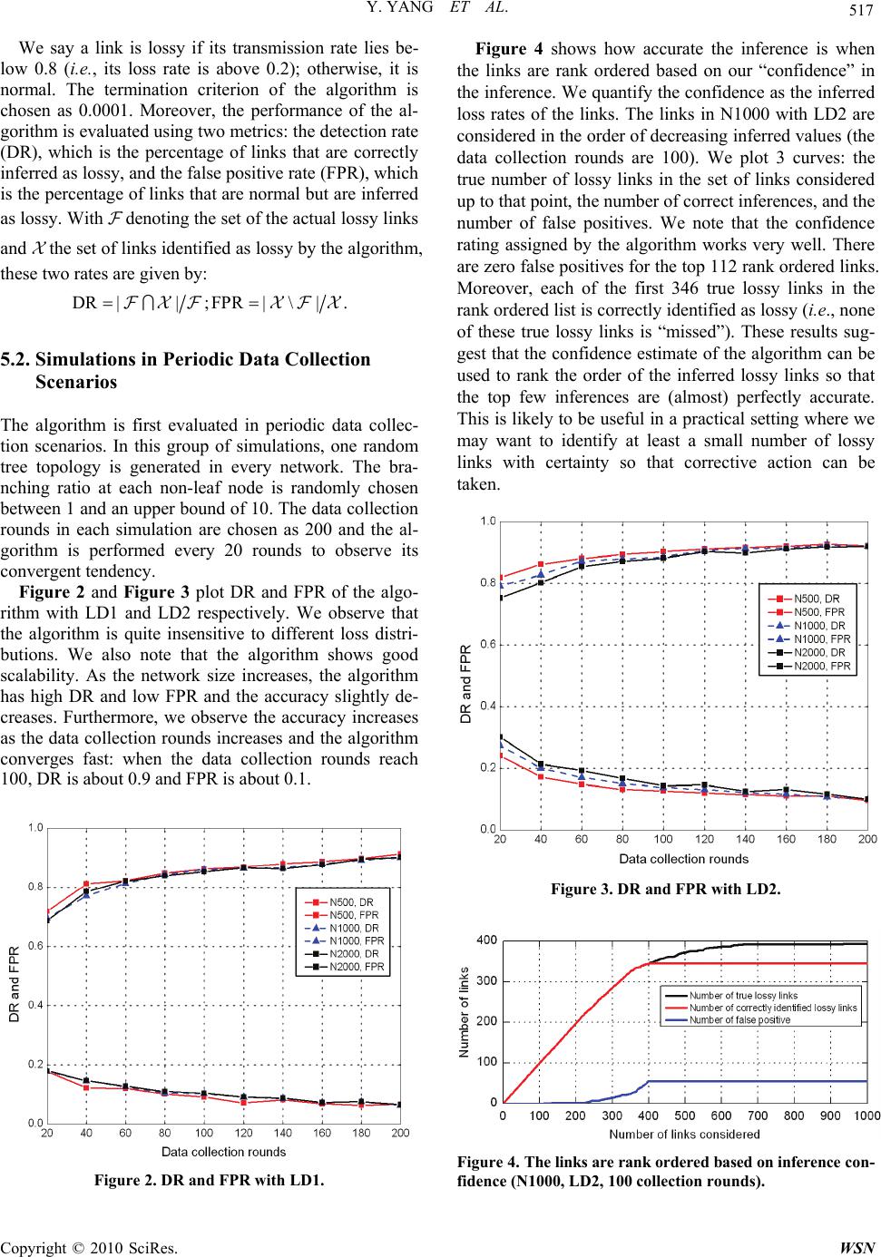

Y. YANG ET AL.
517
We say a link is lossy if its transmission rate lies be-
low 0.8 (i.e., its loss rate is above 0.2); otherwise, it is
normal. The termination criterion of the algorithm is
chosen as 0.0001. Moreover, the performance of the al-
gorithm is evaluated using two metrics: the detection rate
(DR), which is the percentage of links that are correctly
inferred as lossy, and the false positive rate (FPR), which
is the percentage of links that are normal but are inferred
as lossy. With  denoting the set of the actual lossy links
and  the set of links identified as lossy by the algorithm,
these two rates are given by:
DR ||;FPR |\|. 
5.2. Simulations in Periodic Data Collection
Scenarios
The algorithm is first evaluated in periodic data collec-
tion scenarios. In this group of simulations, one random
tree topology is generated in every network. The bra-
nching ratio at each non-leaf node is randomly chosen
between 1 and an upper bound of 10. The data collection
rounds in each simulation are chosen as 200 and the al-
gorithm is performed every 20 rounds to observe its
convergent tendency.
Figure 2 and Figure 3 plot DR and FPR of the algo-
rithm with LD1 and LD2 respectively. We observe that
the algorithm is quite insensitive to different loss distri-
butions. We also note that the algorithm shows good
scalability. As the network size increases, the algorithm
has high DR and low FPR and the accuracy slightly de-
creases. Furthermore, we observe the accuracy increases
as the data collection rounds increases and the algorithm
converges fast: when the data collection rounds reach
100, DR is about 0.9 and FPR is about 0.1.
Figure 2. DR and FPR with LD1.
Figure 4 shows how accurate the inference is when
the links are rank ordered based on our “confidence” in
the inference. We quantify the confidence as the inferred
loss rates of the links. The links in N1000 with LD2 are
considered in the order of decreasing inferred values (the
data collection rounds are 100). We plot 3 curves: the
true number of lossy links in the set of links considered
up to that point, the number of correct inferences, and the
number of false positives. We note that the confidence
rating assigned by the algorithm works very well. There
are zero false positives for the top 112 rank ordered links.
Moreover, each of the first 346 true lossy links in the
rank ordered list is correctly identified as lossy (i.e., none
of these true lossy links is “missed”). These results sug-
gest that the confidence estimate of the algorithm can be
used to rank the order of the inferred lossy links so that
the top few inferences are (almost) perfectly accurate.
This is likely to be useful in a practical setting where we
may want to identify at least a small number of lossy
links with certainty so that corrective action can be
taken.
Figure 3. DR and FPR with LD2.
Figure 4. The links are rank ordered based on inference con-
fidence (N1000, LD2, 100 collection rounds).

Y. YANG ET AL.
518
5.3. Simulations in Events Detection Scenarios
In this section, the algorithm is evaluated in events de-
tection scenarios. The experimental setup of this group of
simulations is as follows. The networks are randomly
placed in a square area of D size and the sink is located
at the upper left corner of the area. The communication
radius of sensor nodes is set as 0.05D. In each experi-
ment, 100 events randomly happen one after another in
the area with the event range S. For each event, a data
aggregation tree is constructed using the greedy incre-
mental tree algorithm proposed in [22] to transmit the
event information to the sink. See Figure 1. After data
collection, the algorithm is performed on the observa-
tions of all trees to obtain the combined results.
The simulations are divided into two groups. The first
group of simulations is used to evaluate the convergence
of the algorithm in events detection scenarios. In this
group the data collection rounds of each aggregation tree
are selected randomly in [0, 50], [50, 100] or [100, 150]
and the event ranges are set as 0.1D. The second group is
used to investigate the performance of our algorithm
with different scales of aggregation trees in events detec-
tion scenarios. In this group the event ranges vary be-
tween 0.05D, 0.1D and 0.15D while the data collection
rounds of each aggregation tree are uniformly distributed
in [50, 100].
Figure 5 and Figure 6 depict the simulation results of
the first group of experiments. The figures suggest that
the algorithm is also robust against different loss distrib-
utions and scales well. Furthermore, the algorithm shows
good convergence: even through the collection rounds of
each tree are less than 50, the algorithm still has high DR
and low FPR. The underlying reason for this success can
be attributed to the fact that for the links that are con-
tained by more than one trees, the algorithm can combine
more observations and therefore the results are more
accurate.
The simulation results of the second group of experi-
ments are illustrated in Figure 7 and Figure 8. We also
note that the algorithm performs similarly under different
Figure 5. DR and FPR with different data collection rounds
of each aggregation tree (LD1).
Figure 6. DR and FPR with different data collection rounds
of each aggregation tree (LD2).
Figure 7. DR and FPR with different event ranges (LD1).
Figure 8. DR and FPR with different event ranges (LD2).
network scales and loss distributions. Moreover, we obs-
erve that its accuracy increases as evnt range, S, inc-
reases. The number of the links that shared by multiple
trees will increase when S increase. Thus the algorithm
can perform more accurately by combining more obser-
vations.
6. Conclusions
In this paper we consider the problem of inferring link
loss rates from the application traffic between sensor no-
des and the sink taken from a collection of aggregation

Y. YANG ET AL.
519
trees. Based on the data aggregation communication par-
adigm, we propose a practical loss performance infer-
ence algorithm using the standard Expectation-Maximi-
zation (EM) techniques. Our algorithm simply observes
the application traffic of the network and handles well
topology changes. Therefore, our approach is applicable
not only to periodic data collection scenarios but also to
events detection scenarios. Via simulations varying be-
tween different network scales, application scenarios,
loss distributions, it can be observed that the algorithm
converges fast and exhibits good scalability and stability.
7. References
[1] C. G. Vehbi and P. H. Gerhard, “Industrial Wireless Sen-
Sor Networks: Challenges, Design Principles, and Tech-
nical Approaches,” IEEE Transactions on Industrial Elec-
tronics, Vol. 56, No. 10, October 2009, pp. 4258-4265.
[2] J. A. Stankovic, “When Sensor and Actuator Networks
Cover the World,” ETRI Journal, Vol. 30, No. 5, October
2008, pp. 627-633.
[3] A. Willig, “Recent and Emerging Topics in Wireless Ind-
ustrial Communications: A Selection,” IEEE Transac-
tions on Industrial Informatics, Vol. 4, No. 2, May 2008,
pp. 102-124.
[4] E. Fasolo, M. Rossi, J. Widmer and M. Zorzi, “In-Net-
work Aggregation Techniques for Wireless Sensor Net-
works: A Survey,” IEEE Wireless Communications, Vol.
14, No. 2, 2007, pp. 70-86.
[5] K. S. Low, W. N. N. Win and M. J. Er, “Wireless Sensor
Networks for Industrial Environments,” Proceedings of
International Conference on Computational Intelligence
for Modelling, Control and International Conference on
Automation and Intelligent Agents, Web Technologies
and Internet Commerce, Vienna, Vol. 2, 2005, pp. 271-
276.
[6] G. J. McLachlan and T. Krishnan, “The EM Algorithm
and Extensions,” 2nd Edition, John Wiley and Sons, Inc,
New York, 2008.
[7] R. Castro, M. Coates, G. Liang, R. Nowak and B. Yu,
“Network Tomography: Recent Developments,” Statisti-
cal Science, Vol. 19, No. 3, 2004, pp. 499-517.
[8] B. Tian, D. Nick, P. Francesco Lo and T. Don, “Network
Tomography on General Topologies,” ACM SIGMET-
RICS Performance Evaluation Review, Vol. 30, No. 1,
2002, pp. 21-30.
[9] S. Rost and H. Balakrishnan, “Memento: A Health Moni-
toring System for Wireless Sensor Networks,” Proceed-
ings of 3rd Annual IEEE Communications Society on
Sensor and Ad Hoc Communications and Networks,
Santa Clara, Vol. 3, 2006, pp. 575-584.
[10] X. Meng, T. Nandagopal, L. Li and S. Lu, “Contour
Maps: Monitoring and Diagnosis in Sensor Networks,”
Computer Networks, Vol. 50, No. 15, 2006, pp. 2820-
2838.
[11] N. Ramanathan, K. Chang, R. Kapur, L. Girod and E.
Kohler, “Sympathy for the Sensor Network Debugger,”
Proceedings of ACM Conference on Embedded Net-
worked Sensor Systems (SenSys), San Diego, 2005, pp.
255-267.
[12] S. Gupta, R. Zheng and A. M. K. Cheng, “ANDES: An
Anomaly Detection System for Wireless Sensor Net-
works,” Proceedings of IEEE International Conference
on Mobile Adhoc and Sensor Systems (MASS), Pisa, 2007,
pp. 1-9.
[13] A. Meier, M. Motani, S. Hu and K. Simon, “DiMo: Dis-
tributed Node Monitoring in Wireless Sensor Networks,”
Proceedings of International Symposium on Modeling,
Analysis and Simulation of Wireless and Mobile Systems,
Vancouver, 2008, pp. 117-121.
[14] G. Hartl and B. Li, “Loss Inference in Wireless Sensor
Networks Based on Data Aggregation,” Proceedings of
International Symposium on Information Processing in
Sensor Networks (IPSN), Berkeley, 2004, pp. 396-404.
[15] Y. Mao, F. R. Kschischang, B. Li and S. Pasupathy, “A
Factor Graph Approach to Link Loss Monitoring in
Wireless Sensor Networks,” IEEE Journal on Selected
Areas in Communications, Vol. 23, No. 4, 2005, pp. 820-
829.
[16] Y. Li, W. Cai, G. Tian and W. Wang, “Loss Tomography
in Wireless Sensor Network Using Gibbs Sampling,”
Proceedings of European Conference on Wireless Sensor
Networks, Delft, 2007, pp. 150-162.
[17] E. Shakshuki and X. Xing, “A Fault Inference Mecha-
nism in Sensor Networks Using Markov Chain,” Pro-
ceedings of the 22nd International Conference on Ad-
vanced Information Networking and Applications, Gi-
noWan, 2008, pp. 628-635.
[18] H. X. Nguyen and P. Thiran, “Using End-To-End Data to
Infer Lossy Links in Sensor Networks,” Proceedings of
IEEE International Conference on Computer Communi-
cations (INFOCOM), Barcelona, 2006, pp. 2205-2216.
[19] K. Liu, M. Li, Y. Liu, M. Li and Z. Guo, “Passive Dia-
Gnosis for Wireless Sensor Networks,” Proceedings of
ACM Conference on Embedded Network Sensor Systems
(SenSys), New York, 2008, pp. 113-126.
[20] B. Wang, W. Wei, W. Zeng and R. P. Krishna, “Fault
Localization Using Passive End-to-End Measurement and
Sequential Testing for Wireless Sensor Networks,” Pro-
ceedings of IEEE Communications Society Conference on
Sensor, Mesh and Ad Hoc Communications and Networks,
Rome, 2009, pp. 225-234.
[21] A. Woo, T. Tong and D. Culler, “Taming the Underlying
Challenges of Reliable Multi-Hop Routing in Sensor Net-
Works,” Proceedings of ACM Conference on Embedded
Networked Sensor Systems, Los Angeles, 2003, pp. 14-
17.
[22] B. Krishnamachari, D. Estrin and S. Wicker, “The Impact
of Data Aggregation in Wireless Sensor Networks,” Pro-
ceedings of the 22nd International Conference on Dis-
tributed Computing Systems, Vienna, 2002, pp. 575-578.