Paper Menu >>
Journal Menu >>
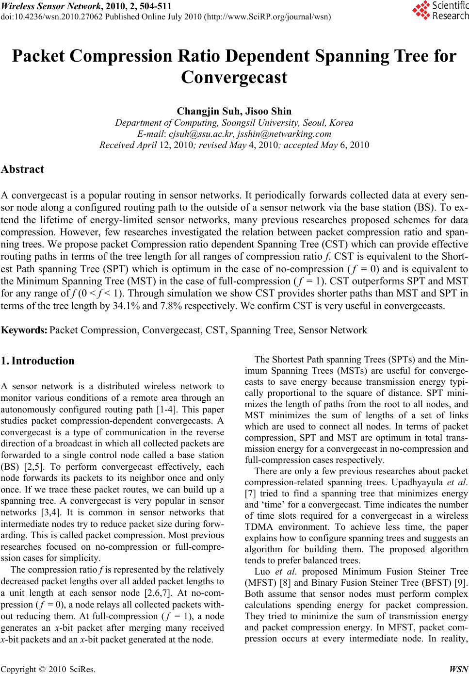 Wireless Sensor Network, 2010, 2, 504-511 doi:10.4236/wsn.2010.27062 Published Online July 2010 (http://www.SciRP.org/journal/wsn) Copyright © 2010 SciRes. WSN Packet Compression Ratio Dependent Spanning Tree for Convergecast Changjin Suh, Jisoo Shin Department of Computing, Soongsil University, Seoul, Korea E-mail: cjsuh@ssu.ac.kr, jsshin@netwarking.com Received April 12, 2010; revised May 4, 2010; accepted May 6, 2010 Abstract A convergecast is a popular routing in sensor networks. It periodically forwards collected data at every sen- sor node along a configured routing path to the outside of a sensor network via the base station (BS). To ex- tend the lifetime of energy-limited sensor networks, many previous researches proposed schemes for data compression. However, few researches investigated the relation between packet compression ratio and span- ning trees. We propose packet Compression ratio dependent Spanning Tree (CST) which can provide effective routing paths in terms of the tree length for all ranges of compression ratio f. CST is equivalent to the Short- est Path spanning Tree (SPT) which is optimum in the case of no-compression (f = 0) and is equivalent to the Minimum Spanning Tree (MST) in the case of full-compression (f = 1). CST outperforms SPT and MST for any range of f (0 < f < 1). Through simulation we show CST provides shorter paths than MST and SPT in terms of the tree length by 34.1% and 7.8% respectively. We confirm CST is very useful in convergecasts. Keywords: Packet Compression, Convergecast, CST, Spanning Tree, Sensor Network 1. Introduction A sensor network is a distributed wireless network to monitor various conditions of a remote area through an autonomously configured routing path [1-4]. This paper studies packet compression-dependent convergecasts. A convergecast is a type of communication in the reverse direction of a broadcast in which all collected packets are forwarded to a single control node called a base station (BS) [2,5]. To perform convergecast effectively, each node forwards its packets to its neighbor once and only once. If we trace these packet routes, we can build up a spanning tree. A convergecast is very popular in sensor networks [3,4]. It is common in sensor networks that intermediate nodes try to reduce packet size during forw- arding. This is called packet compression. Most previous researches focused on no-compression or full-compre- ssion cases for simplicity. The compression ratio f is represented by the relatively decreased packet lengths over all added packet lengths to a unit length at each sensor node [2,6,7]. At no-com- pression (f = 0), a node relays all collected packets with- out reducing them. At full-compression (f = 1), a node generates an x-bit packet after merging many received x-bit packets and an x-bit packet generated at the node. The Shortest Path spanning Trees (SPTs) and the Min- imum Spanning Trees (MSTs) are useful for converge- casts to save energy because transmission energy typi- cally proportional to the square of distance. SPT mini- mizes the length of paths from the root to all nodes, and MST minimizes the sum of lengths of a set of links which are used to connect all nodes. In terms of packet compression, SPT and MST are optimum in total trans- mission energy for a convergecast in no-compression and full-compression cases respectively. There are only a few previous researches about packet compression-related spanning trees. Upadhyayula et al. [7] tried to find a spanning tree that minimizes energy and ‘time’ for a convergecast. Time indicates the number of time slots required for a convergecast in a wireless TDMA environment. To achieve less time, the paper explains how to configure spanning trees and suggests an algorithm for building them. The proposed algorithm tends to prefer balanced trees. Luo et al. proposed Minimum Fusion Steiner Tree (MFST) [8] and Binary Fusion Steiner Tree (BFST) [9]. Both assume that sensor nodes must perform complex calculations spending energy for packet compression. They tried to minimize the sum of transmission energy and packet compression energy. In MFST, packet com- pression occurs at every intermediate node. In reality, 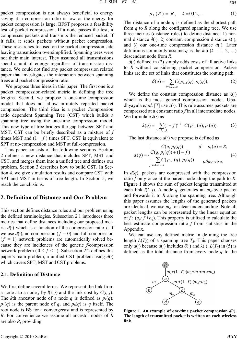 C. J. SUH ET AL. Copyright © 2010 SciRes. WSN 505 packet compression is not always beneficial to energy saving if a compression ratio is low or the energy for packet compression is large. BFST proposes a feasibility test of packet compression. If a node passes the test, it compresses packets and transmits the reduced packet. If it fails, it sends packets without packet compression. These researches focused on the packet compression side, leaving transmission oversimplified. Spanning trees were not their main interest. They assumed all transmissions spend a unit of energy regardless of transmission dis- tance. We could not find any packet compression related paper that investigates the interaction between spanning trees and packet compression ratio. We propose three ideas in this paper. The first one is a packet compression-related metric in defining the tree lengths. Second, we propose a one-time compression model that does not allow infinitely repeated packet compression. The third idea is a packet Compression ratio dependent Spanning Tree (CST) which builds a spanning tree using the one-time compression model. This new type of tree bridges the gap between SPT and MST. CST can be briefly described as a mixture of f times MST and (1 − f ) times SPT. CST is equivalent to SPT at no-compression and MST at full-compression. This paper consists of the following sections. Section 2 defines a new distance that includes SPT, MST and CST, and merges them into a unified tree and defines our problem. Section 3 describes how to build CST. In Sec- tion 4, we give simulation results and compare CST with SPT and MST in terms of tree length. In Section 5, we reach the conclusions. 2. Definition of Distance and Our Problem This section defines distance rules and our problem using the defined terminologies. Subsection 2.1 introduces three metrics that define distances including our proposed met- ric d(·) which is a function of the compression ratio f. If we use d(·), no-compression (f = 0) and full-compression (f = 1) network problems are automatically solved be- cause they are incidences of the generic f-compression network problem (10 f). Subsection 2.2 defines this paper’s main problem, a unified CST problem using d(·) which covers SPT, MST and CST problems. 2.1. Definition of Distance We first define several terms. We represent the link from a node i to a node j by l(i, j) and the link cost by C(i, j). The kth ancestor node of a node q is defined as pk(q). p1(q) is the parent node of q, and p0(q) is q itself. The root node is BS for a convergecast and is represented by R. For convenience we assume all ancestor nodes of R are also R, providing: ,)( RRpk ,....2,1,0k (1) The distance of a node q is defined as the shortest path from q to R along the configured spanning tree. We use three metrics (distance rules) to define distance: 1) nor- mal distance δ(·), 2) constant compression distance λ(·), and 3) our one-time compression distance d(·). Later definitions commonly assume q is the kth (k = 1, 2, …) descendent node from R. δ(·) defined in (2) simply adds costs of all active links to R without considering packet compression. Active links are the set of links that constitutes the routing path. ki iiqpqpCq ,...,2,1 1)).(),(()( (2) We define the constant compression distance as λ(·) which is the most general compression model. Upa- dhyayula et al. [7] use λ(·). This rule assumes packets are compressed at a constant ratio f in all intermediate nodes. We formulate λ(·) as ki ii iqpqpCfq ,...,2,1 1 1)).(),(()1()( (3) The last distance d(·) we propose is defined as . ))(),(( )1())(,( ,)())(,( )( ,...,2,1 1 1 11 otherwise qpqpC fqpqC RqpifqpqC qd ki ii (4) In d(q), packets are compressed with the compression ratio f only once at the parent node along the path to R. Figure 1 shows the sum of packet lengths transmitted at each link l(i, j). A node q generates an mq-byte packet and forwards it to R along the spanning tree. Although this paper assumes the lengths of the generated packets are identical, we use mq for clear understanding. Note all packet lengths can be represented by the linear equation of f : (aij· f +bij). This property is utilized to calculate the best estimate compression ratio f from statistics in the Appendix. We can use any defined metric in defining the tree length L(TS) of a spanning tree TS. This paper chooses only d(·) because d(·) includes δ(·) and λ(·). L(TS) in (5) is defined as the total distance from every node q to the Figure 1. An example of one-time packet compression d(·). The length of transmitted packet is written on each wireless link. 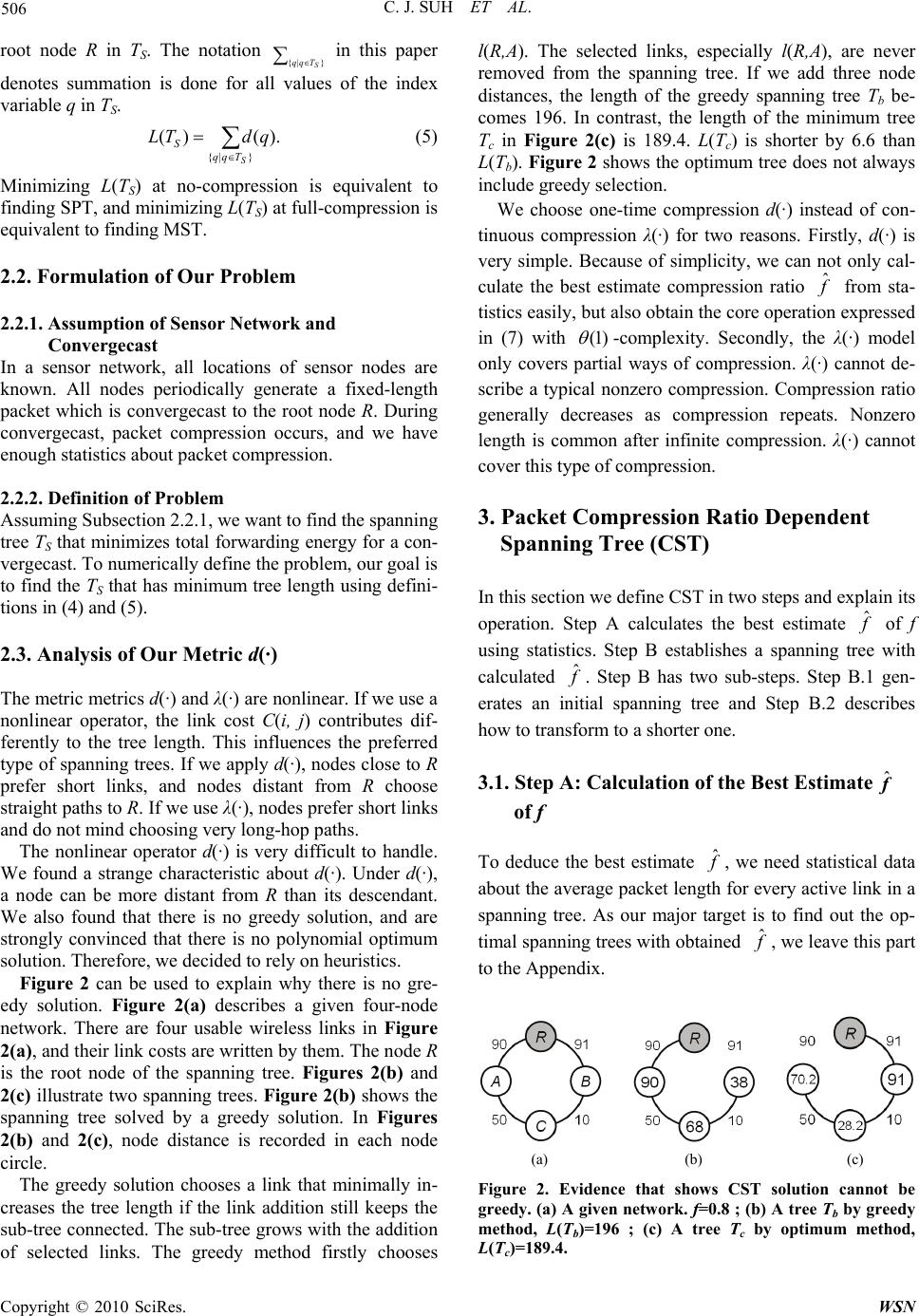 C. J. SUH ET AL. Copyright © 2010 SciRes. WSN 506 root node R in TS. The notation }|{ S Tqq in this paper denotes summation is done for all values of the index variable q in TS. }|{ ).()( S Tqq SqdTL (5) Minimizing L(TS) at no-compression is equivalent to finding SPT, and minimizing L(TS) at full-compression is equivalent to finding MST. 2.2. Formulation of Our Problem 2.2.1. Assumption of Sensor Network and Convergecast In a sensor network, all locations of sensor nodes are known. All nodes periodically generate a fixed-length packet which is convergecast to the root node R. During convergecast, packet compression occurs, and we have enough statistics about packet compression. 2.2.2. Definition of Problem Assuming Subsection 2.2.1, we want to find the spanning tree TS that minimizes total forwarding energy for a con- vergecast. To numerically define the problem, our goal is to find the TS that has minimum tree length using defini- tions in (4) and (5). 2.3. Analysis of Our Metric d(·) The metric metrics d(·) and λ(·) are nonlinear. If we use a nonlinear operator, the link cost C(i, j) contributes dif- ferently to the tree length. This influences the preferred type of spanning trees. If we apply d(·), nodes close to R prefer short links, and nodes distant from R choose straight paths to R. If we use λ(·), nodes prefer short links and do not mind choosing very long-hop paths. The nonlinear operator d(·) is very difficult to handle. We found a strange characteristic about d(·). Under d(·), a node can be more distant from R than its descendant. We also found that there is no greedy solution, and are strongly convinced that there is no polynomial optimum solution. Therefore, we decided to rely on heuristics. Figure 2 can be used to explain why there is no gre- edy solution. Figure 2(a) describes a given four-node network. There are four usable wireless links in Figure 2(a), and their link costs are written by them. The node R is the root node of the spanning tree. Figures 2(b) and 2(c) illustrate two spanning trees. Figure 2(b) shows the spanning tree solved by a greedy solution. In Figures 2(b) and 2(c), node distance is recorded in each node circle. The greedy solution chooses a link that minimally in- creases the tree length if the link addition still keeps the sub-tree connected. The sub-tree grows with the addition of selected links. The greedy method firstly chooses l(R,A). The selected links, especially l(R,A), are never removed from the spanning tree. If we add three node distances, the length of the greedy spanning tree Tb be- comes 196. In contrast, the length of the minimum tree Tc in Figure 2(c) is 189.4. L(Tc) is shorter by 6.6 than L(Tb). Figure 2 shows the optimum tree does not always include greedy selection. We choose one-time compression d(·) instead of con- tinuous compression λ(·) for two reasons. Firstly, d(·) is very simple. Because of simplicity, we can not only cal- culate the best estimate compression ratio f ˆ from sta- tistics easily, but also obtain the core operation expressed in (7) with )1( -complexity. Secondly, the λ(·) model only covers partial ways of compression. λ(·) cannot de- scribe a typical nonzero compression. Compression ratio generally decreases as compression repeats. Nonzero length is common after infinite compression. λ(·) cannot cover this type of compression. 3. Packet Compression Ratio Dependent Spanning Tree (CST) In this section we define CST in two steps and explain its operation. Step A calculates the best estimate f ˆ of f using statistics. Step B establishes a spanning tree with calculated f ˆ. Step B has two sub-steps. Step B.1 gen- erates an initial spanning tree and Step B.2 describes how to transform to a shorter one. 3.1. Step A: Calculation of the Best Estimate f ˆ of f To deduce the best estimate f ˆ, we need statistical data about the average packet length for every active link in a spanning tree. As our major target is to find out the op- timal spanning trees with obtained f ˆ, we leave this part to the Appendix. (a) (b) (c) Figure 2. Evidence that shows CST solution cannot be greedy. (a) A given network. f=0.8 ; (b) A tree Tb by greedy method, L(Tb)=196 ; (c) A tree Tc by optimum method, L(Tc)=189.4. 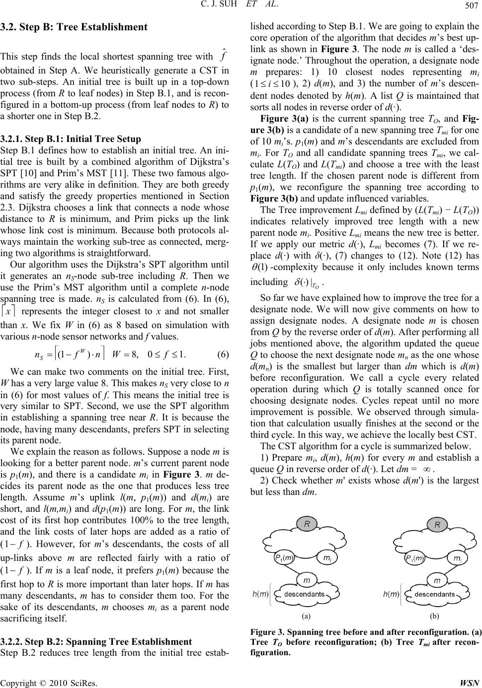 C. J. SUH ET AL. Copyright © 2010 SciRes. WSN 507 3.2. Step B: Tree Establishment This step finds the local shortest spanning tree with f ˆ obtained in Step A. We heuristically generate a CST in two sub-steps. An initial tree is built up in a top-down process (from R to leaf nodes) in Step B.1, and is recon- figured in a bottom-up process (from leaf nodes to R) to a shorter one in Step B.2. 3.2.1. Step B.1: Initial Tree Setup Step B.1 defines how to establish an initial tree. An ini- tial tree is built by a combined algorithm of Dijkstra’s SPT [10] and Prim’s MST [11]. These two famous algo- rithms are very alike in definition. They are both greedy and satisfy the greedy properties mentioned in Section 2.3. Dijkstra chooses a link that connects a node whose distance to R is minimum, and Prim picks up the link whose link cost is minimum. Because both protocols al- ways maintain the working sub-tree as connected, merg- ing two algorithms is straightforward. Our algorithm uses the Dijkstra’s SPT algorithm until it generates an nS-node sub-tree including R. Then we use the Prim’s MST algorithm until a complete n-node spanning tree is made. nS is calculated from (6). In (6), x represents the integer closest to x and not smaller than x. We fix W in (6) as 8 based on simulation with various n-node sensor networks and f values. nfn W S)1( ,8 W .10 f (6) We can make two comments on the initial tree. First, W has a very large value 8. This makes nS very close to n in (6) for most values of f. This means the initial tree is very similar to SPT. Second, we use the SPT algorithm in establishing a spanning tree near R. It is because the node, having many descendants, prefers SPT in selecting its parent node. We explain the reason as follows. Suppose a node m is looking for a better parent node. m’s current parent node is p1(m), and there is a candidate mi in Figure 3. m de- cides its parent node as the one that produces less tree length. Assume m’s uplink l(m, p 1(m)) and d(mi) are short, and l(m,mi) and d(p1(m)) are long. For m, the link cost of its first hop contributes 100% to the tree length, and the link costs of later hops are added as a ratio of (f1). However, for m’s descendants, the costs of all up-links above m are reflected fairly with a ratio of (f1). If m is a leaf node, it prefers p1(m) because the first hop to R is more important than later hops. If m has many descendants, m has to consider them too. For the sake of its descendants, m chooses mi as a parent node sacrificing itself. 3.2.2. Step B.2: Spanning Tree Establishment Step B.2 reduces tree length from the initial tree estab- lished according to Step B.1. We are going to explain the core operation of the algorithm that decides m’s best up- link as shown in Figure 3. The node m is called a ‘des- ignate node.’ Throughout the operation, a designate node m prepares: 1) 10 closest nodes representing mi (101 i), 2) d(m), and 3) the number of m’s descen- dent nodes denoted by h(m). A list Q is maintained that sorts all nodes in reverse order of d(·). Figure 3(a) is the current spanning tree TO, and Fig- ure 3(b) is a candidate of a new spanning tree Tmi for one of 10 mi’s. p1(m) and m’s descendants are excluded from mi. For TO and all candidate spanning trees Tmi, we cal- culate L(TO) and L(Tmi) and choose a tree with the least tree length. If the chosen parent node is different from p1(m), we reconfigure the spanning tree according to Figure 3(b) and update influenced variables. The Tree improvement Lmi defined by (L(Tmi) − L(TO)) indicates relatively improved tree length with a new parent node mi. Positive Lmi means the new tree is better. If we apply our metric d(·), Lmi becomes (7). If we re- place d(·) with δ(·), (7) changes to (12). Note (12) has )1( -complexity because it only includes known terms including O T |)( . So far we have explained how to improve the tree for a designate node. We will now give comments on how to assign designate nodes. A designate node m is chosen from Q by the reverse order of d(m). After performing all jobs mentioned above, the algorithm updated the queue Q to choose the next designate node mn as the one whose d(mn) is the smallest but larger than dm which is d(m) before reconfiguration. We call a cycle every related operation during which Q is totally scanned once for choosing designate nodes. Cycles repeat until no more improvement is possible. We observed through simula- tion that calculation usually finishes at the second or the third cycle. In this way, we achieve the locally best CST. The CST algorithm for a cycle is summarized below. 1) Prepare mi, d(m), h(m) for every m and establish a queue Q in reverse order of d(·). Let dm = . 2) Check whether m' exists whose d(m') is the largest but less than dm. (a) (b) Figure 3. Spanning tree before and after reconfiguration. (a) Tree TO before reconfiguration; (b) Tree Tmi after recon- figuration. 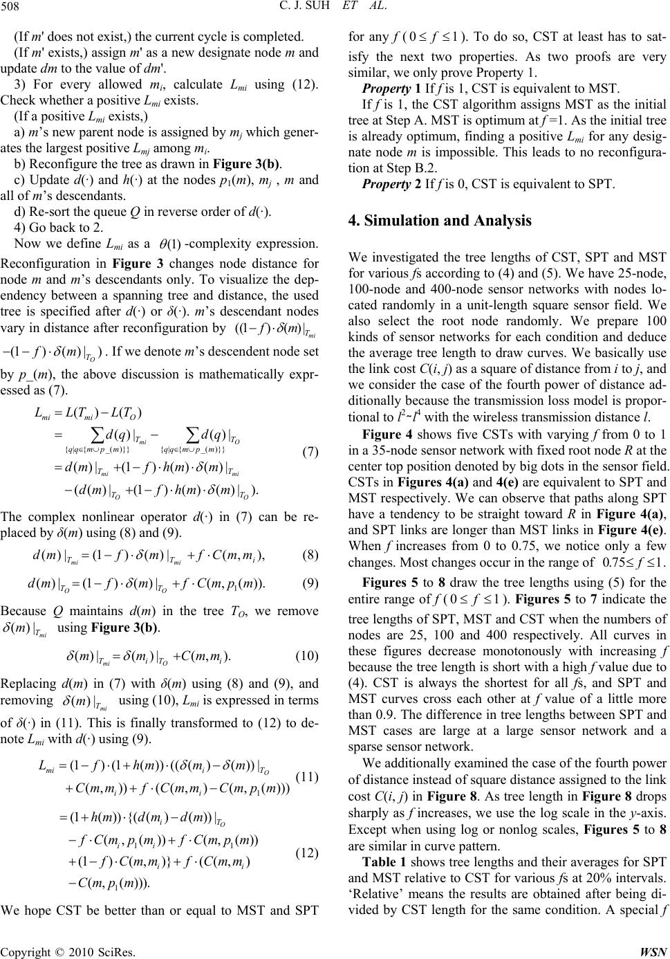 C. J. SUH ET AL. Copyright © 2010 SciRes. WSN 508 (If m' does not exist,) the current cycle is completed. (If m' exists,) assign m' as a new designate node m and update dm to the value of dm'. 3) For every allowed mi, calculate Lmi using (12). Check whether a positive Lmi exists. (If a positive Lmi exists,) a) m’s new parent node is assigned by mj which gener- ates the largest positive Lmj among mi. b) Reconfigure the tree as drawn in Figure 3(b). c) Update d(·) and h(·) at the nodes p1(m), mj , m and all of m’s descendants. d) Re-sort the queue Q in reverse order of d(·). 4) Go back to 2. Now we define Lmi as a )1( -complexity expression. Reconfiguration in Figure 3 changes node distance for node m and m’s descendants only. To visualize the dep- endency between a spanning tree and distance, the used tree is specified after d(·) or δ(·). m’s descendant nodes vary in distance after reconfiguration by mi T mf |)()1(( )|)()1( O T mf . If we denote m’s descendent node set by p_(m), the above discussion is mathematically expr- essed as (7). ).|)()()1(|)(( |)()()1(|)( |)(|)( )()( )}}_({|{)}}_({|{ OO mimi Omi TT TT mpmqq T mpmqq T Omimi mmhfmd mmhfmd qdqd TLTLL (7) The complex nonlinear operator d(·) in (7) can be re- placed by δ(m) using (8) and (9). ),,(|)()1(|)( iTTmmCfmfmd mimi (8) )).(,(|)()1(|)( 1mpmCfmfmd OO TT (9) Because Q maintains d(m) in the tree TO, we remove mi T m|)( using Figure 3(b). ).,(|)(|)( iTiT mmCmm Omi (10) Replacing d(m) in (7) with δ(m) using (8) and (9), and removing mi T m|)( using (10), Lmi is expressed in terms of δ(·) in (11). This is finally transformed to (12) to de- note Lmi with d(·) using (9). )))(,(),(()),( |))()((())(1()1( 1mpmCmmCfmmC mmmhfL ii Timi O (11) 11 1 (1()){(()())| (,())(,()) (1)(,)}((,) (,())). O iT ii ii hmdm dm f Cmp mfCmp m fCmm fCmm Cmp m (12) We hope CST be better than or equal to MST and SPT for any f (10 f). To do so, CST at least has to sat- isfy the next two properties. As two proofs are very similar, we only prove Property 1. Property 1 If f is 1, CST is equivalent to MST. If f is 1, the CST algorithm assigns MST as the initial tree at Step A. MST is optimum at f =1. As the initial tree is already optimum, finding a positive Lmi for any desig- nate node m is impossible. This leads to no reconfigura- tion at Step B.2. Property 2 If f is 0, CST is equivalent to SPT. 4. Simulation and Analysis We investigated the tree lengths of CST, SPT and MST for various fs according to (4) and (5). We have 25-node, 100-node and 400-node sensor networks with nodes lo- cated randomly in a unit-length square sensor field. We also select the root node randomly. We prepare 100 kinds of sensor networks for each condition and deduce the average tree length to draw curves. We basically use the link cost C(i, j) as a square of distance from i to j, and we consider the case of the fourth power of distance ad- ditionally because the transmission loss model is propor- tional to l2∼l4 with the wireless transmission distance l. Figure 4 shows five CSTs with varying f from 0 to 1 in a 35-node sensor network with fixed root node R at the center top position denoted by big dots in the sensor field. CSTs in Figures 4(a) and 4(e) are equivalent to SPT and MST respectively. We can observe that paths along SPT have a tendency to be straight toward R in Figure 4(a), and SPT links are longer than MST links in Figure 4(e). When f increases from 0 to 0.75, we notice only a few changes. Most changes occur in the range of 175.0 f. Figures 5 to 8 draw the tree lengths using (5) for the entire range of f (10 f). Figures 5 to 7 indicate the tree lengths of SPT, MST and CST when the numbers of nodes are 25, 100 and 400 respectively. All curves in these figures decrease monotonously with increasing f because the tree length is short with a high f value due to (4). CST is always the shortest for all fs, and SPT and MST curves cross each other at f value of a little more than 0.9. The difference in tree lengths between SPT and MST cases are large at a large sensor network and a sparse sensor network. We additionally examined the case of the fourth power of distance instead of square distance assigned to the link cost C(i, j) in Figure 8. As tree length in Figure 8 drops sharply as f increases, we use the log scale in the y-axis. Except when using log or nonlog scales, Figures 5 to 8 are similar in curve pattern. Table 1 shows tree lengths and their averages for SPT and MST relative to CST for various fs at 20% intervals. ‘Relative’ means the results are obtained after being di- vided by CST length for the same condition. A special f 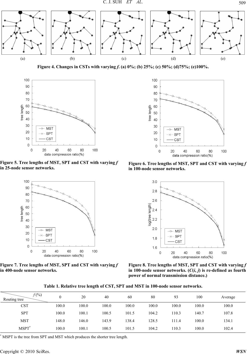 C. J. SUH ET AL. Copyright © 2010 SciRes. WSN 509 (a) (b) (c) (d) (e) Figure 4. Changes in CSTs with varying f. (a) 0%; (b) 25%; (c) 50%; (d)75%; (e)100%. Figure 5. Tree lengths of MST, SPT and CST with varying f in 25-node sensor networks. Figure 6. Tree lengths of MST, SPT and CST with varying f in 100-node sensor networks. Figure 7. Tree lengths of MST, SPT and CST with varying f in 400-node sensor networks. Figure 8. Tree lengths of MST, SPT and CST with varying f in 100-node sensor networks. (C(i, j) is re-defined as fourth power of normal transmission distance.) Table 1. Relative tree length of CST, SPT and MST in 100-node sensor networks. f (%) Routing tree 0 20 40 60 80 93 100 Average CST 100.0 100.0 100.0 100.0 100.0 100.0 100.0 100.0 SPT 100.0 100.1 100.5 101.5 104.2 110.3 140.7 107.8 MST 148.0 146.0 143.9 138.4 128.5 111.4 100.0 134.1 MSPT* 100.0 100.1 100.5 101.5 104.2 110.3 100.0 102.4 * MSPT is the tree from SPT and MST which produces the shorter tree length. 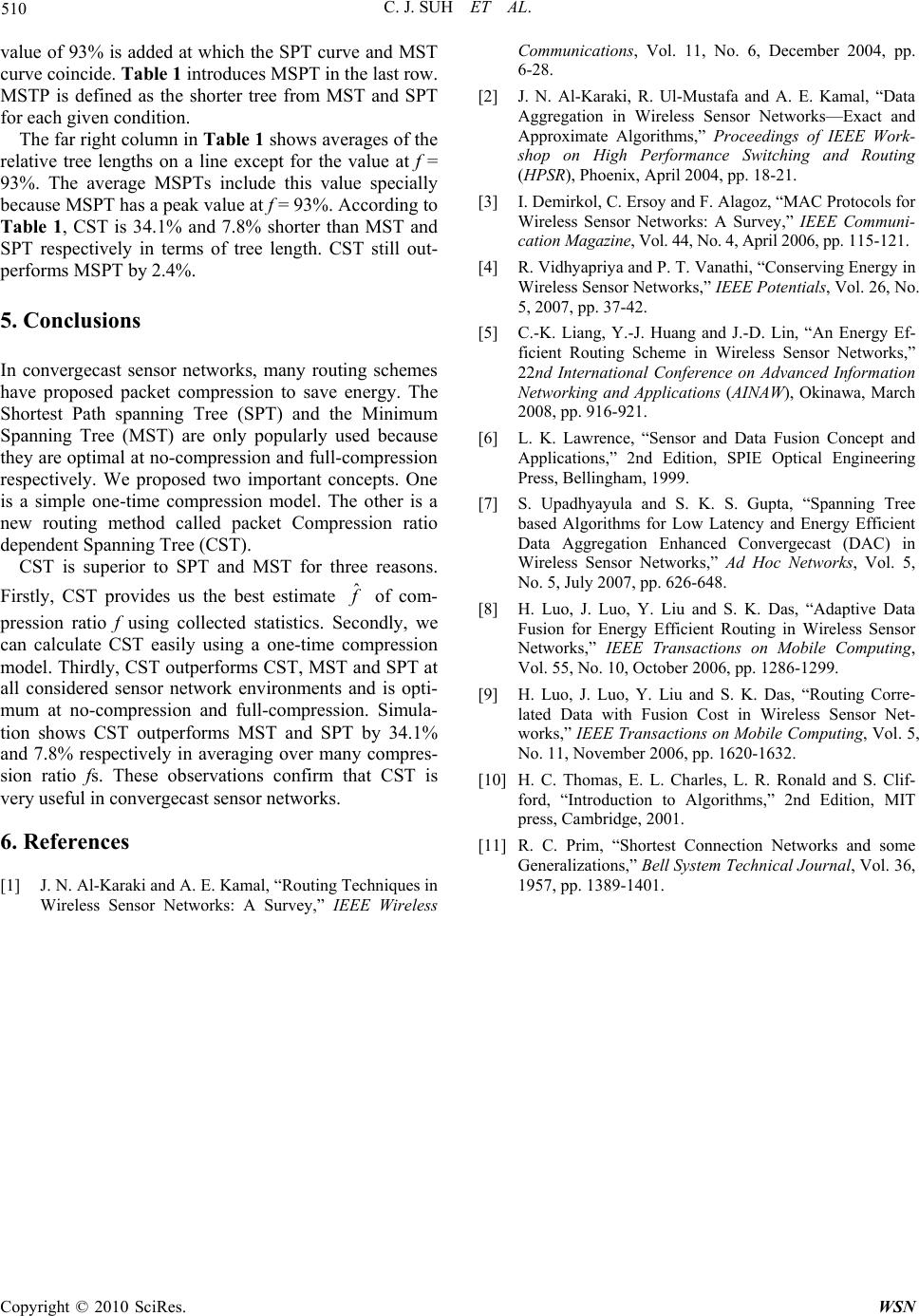 C. J. SUH ET AL. Copyright © 2010 SciRes. WSN 510 value of 93% is added at which the SPT curve and MST curve coincide. Table 1 introduces MSPT in the last row. MSTP is defined as the shorter tree from MST and SPT for each given condition. The far right column in Table 1 shows averages of the relative tree lengths on a line except for the value at f = 93%. The average MSPTs include this value specially because MSPT has a peak value at f = 93%. According to Table 1, CST is 34.1% and 7.8% shorter than MST and SPT respectively in terms of tree length. CST still out- performs MSPT by 2.4%. 5. Conclusions In convergecast sensor networks, many routing schemes have proposed packet compression to save energy. The Shortest Path spanning Tree (SPT) and the Minimum Spanning Tree (MST) are only popularly used because they are optimal at no-compression and full-compression respectively. We proposed two important concepts. One is a simple one-time compression model. The other is a new routing method called packet Compression ratio dependent Spanning Tree (CST). CST is superior to SPT and MST for three reasons. Firstly, CST provides us the best estimate f ˆ of com- pression ratio f using collected statistics. Secondly, we can calculate CST easily using a one-time compression model. Thirdly, CST outperforms CST, MST and SPT at all considered sensor network environments and is opti- mum at no-compression and full-compression. Simula- tion shows CST outperforms MST and SPT by 34.1% and 7.8% respectively in averaging over many compres- sion ratio fs. These observations confirm that CST is very useful in convergecast sensor networks. 6. References [1] J. N. Al-Karaki and A. E. Kamal, “Routing Techniques in Wireless Sensor Networks: A Survey,” IEEE Wireless Communications, Vol. 11, No. 6, December 2004, pp. 6-28. [2] J. N. Al-Karaki, R. Ul-Mustafa and A. E. Kamal, “Data Aggregation in Wireless Sensor Networks—Exact and Approximate Algorithms,” Proceedings of IEEE Work- shop on High Performance Switching and Routing (HPSR), Phoenix, April 2004, pp. 18-21. [3] I. Demirkol, C. Ersoy and F. Alagoz, “MAC Protocols for Wireless Sensor Networks: A Survey,” IEEE Communi- cation Magazine, Vol. 44, No. 4, April 2006, pp. 115-121. [4] R. Vidhyapriya and P. T. Vanathi, “Conserving Energy in Wireless Sensor Networks,” IEEE Potentials, Vol. 26, No. 5, 2007, pp. 37-42. [5] C.-K. Liang, Y.-J. Huang and J.-D. Lin, “An Energy Ef- ficient Routing Scheme in Wireless Sensor Networks,” 22nd International Conference on Advanced Information Networking and Applications (AINAW), Okinawa, March 2008, pp. 916-921. [6] L. K. Lawrence, “Sensor and Data Fusion Concept and Applications,” 2nd Edition, SPIE Optical Engineering Press, Bellingham, 1999. [7] S. Upadhyayula and S. K. S. Gupta, “Spanning Tree based Algorithms for Low Latency and Energy Efficient Data Aggregation Enhanced Convergecast (DAC) in Wireless Sensor Networks,” Ad Hoc Networks, Vol. 5, No. 5, July 2007, pp. 626-648. [8] H. Luo, J. Luo, Y. Liu and S. K. Das, “Adaptive Data Fusion for Energy Efficient Routing in Wireless Sensor Networks,” IEEE Transactions on Mobile Computing, Vol. 55, No. 10, October 2006, pp. 1286-1299. [9] H. Luo, J. Luo, Y. Liu and S. K. Das, “Routing Corre- lated Data with Fusion Cost in Wireless Sensor Net- works,” IEEE Transactions on Mobile Computing, Vol. 5, No. 11, November 2006, pp. 1620-1632. [10] H. C. Thomas, E. L. Charles, L. R. Ronald and S. Clif- ford, “Introduction to Algorithms,” 2nd Edition, MIT press, Cambridge, 2001. [11] R. C. Prim, “Shortest Connection Networks and some Generalizations,” Bell System Technical Journal, Vol. 36, 1957, pp. 1389-1401. 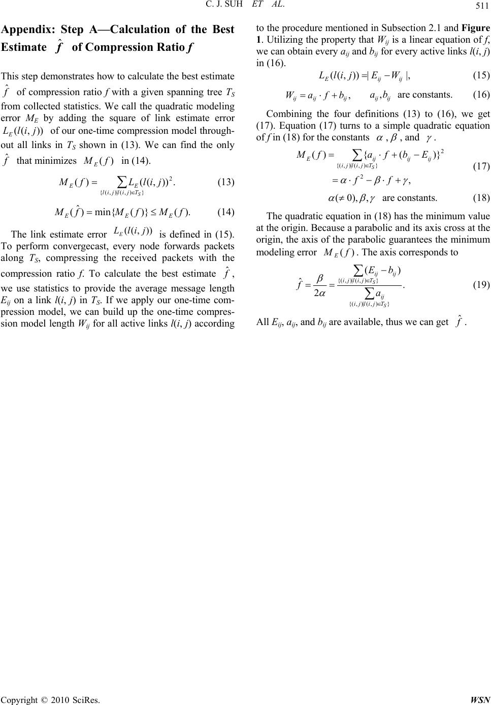 C. J. SUH ET AL. Copyright © 2010 SciRes. WSN 511 Appendix: Step A—Calculation of the Best Estimate f ˆ of Compression Ratio f This step demonstrates how to calculate the best estimate f ˆ of compression ratio f with a given spanning tree TS from collected statistics. We call the quadratic modeling error ME by adding the square of link estimate error )),(( jilLE of our one-time compression model through- out all links in TS shown in (13). We can find the only f ˆ that minimizes )( fM E in (14). .)),(()( }),(|),({ 2 S Tjiljil EE jilLfM (13) ).()}(min{) ˆ (fMfMfM EEE (14) The link estimate error )),(( jilLE is defined in (15). To perform convergecast, every node forwards packets along TS, compressing the received packets with the compression ratio f. To calculate the best estimate f ˆ, we use statistics to provide the average message length Eij on a link l(i, j) in TS. If we apply our one-time com- pression model, we can build up the one-time compres- sion model length Wij for all active links l(i, j) according to the procedure mentioned in Subsection 2.1 and Figure 1. Utilizing the property that Wij is a linear equation of f, we can obtain every aij and bij for every active links l(i, j) in (16). |,|)),(( ijijE WEjilL (15) , ijijij bfaW ijij ba , are constants. (16) Combining the four definitions (13) to (16), we get (17). Equation (17) turns to a simple quadratic equation of f in (18) for the constants , , and . , )}({)( 2 }),(|),{( 2 ff EbfafM S Tjilji ijijijE (17) ,),0( are constants. (18) The quadratic equation in (18) has the minimum value at the origin. Because a parabolic and its axis cross at the origin, the axis of the parabolic guarantees the minimum modeling error )( fM E. The axis corresponds to . )( 2 ˆ }),(|),{( }),(|),{( S S Tjilji ij Tjilji ijij a bE f (19) All Eij, aij, and bij are available, thus we can get f ˆ. |