 Vol.2, No.6, 612-625 (2010) Natural Science http://dx.doi.org/10.4236/ns.2010.26076 Copyright © 2010 SciRes. OPEN ACCESS Application of variational iteration method and electron transfer mediator/catalyst composites in modified electrodes Alagu Eswari, Lakshmanan Rajendran* The Madura College, Madurai, India; *Corresponding Author: raj_sms@rediffmail.com Received 20 February 2010; revised 23 March 2010; accepted 23 April 2010. ABSTRACT The nonlinear coupled system of diffusion equ- ations are solved analytically for the transport and kinetics of electrons and reactant in the layer of a modified electrode. Analytical expres- sions of concentrations of substrate and me- diator are presented using He’s variational itera- tion method. The approximate expression of cu- rrent for microheterogeneous catalysis at iso- nomer or redox polymer modified electrodes is also obtained. The results of the available limit- ing cases are compared with our results and are found to be in good agreement. Keywords: Variational Methods; Nonlinear Boundary Value Problems; Simulation; Reaction-Diffusion Equations; Mathematical Modeling 1. INTRODUCTION Recently the electrocatalytic activity of polymer modi- fied electrodes has been the subject of considerable study of many researchers. Generally most systems are used to require an efficient electron transfer mediator in addition to displaying good electrocatalytic activity. We can find many features for electrocatalysis in the use of microscopic particles of metals or metal oxides disp- ersed within polymeric films deposited on electrode sur- faces. This dispersion of catalytic materials offers im- portant catalytic advantages. We are interested in the design of such microheterogeneous systems for efficient electrocatalysis. A modified electrode differs from an ordinary electr- ode by having a thin film of some coated material which prevent direct contact between the metal surface and the bulk electrolyte. Electrochemical reactions of species in solution take place through that thin film. Instead of a direct electron transfer between the Fermi level of the metal and the ion in solution, the electron transfer is ‘mediated’ by the redox groups present in the thin layer. A large number of different modified electrodes have been made and certain systems have received more at- tention than others. Lyons, McCormack, and Bartlett [1] presented an analytical model which quantified the transport and ki- netics in conducting polymer modified electrodes con- taining a homogeneous distribution of spherical mi- croparticulate catalysts. In their paper Lyons, McCor- mack, and Bartlett [1] obtained the analytical expres- sions of the substrate and mediator concentrations for the different values of parameters. Lyons and Bartlett [2] also presented the analytical expressions of substrate and mediator concentrations only for limiting values of di- mensionless parameters. The transport and kinetics of reactions in chemically modified electrodes have been analyzed previously by Lyons and co-workers and ap- proximate analytical solutions are available [3-7] . In this paper we analyze application of catalyst com- posites in modified electrodes. To date many researches have been done on the application of modified electrodes. To my knowledge no rigorous analytical solutions for substrate and mediator concentrations have been re- ported in that application. Hence the main objective of this paper is to derive the analytical expressions of con- centrations of substrate and mediator for all values of parameters using variational iteration method. The ap- proximate expression of current for microheterogeneous catalysis at isonomer or redox polymer modified elec- trodes is also obtained for all values of dimensionless parameters and (these parameters are defined in the (7)). 2. MATHEMATICAL FORMULATION OF THE PROBLEM AND ANALYSIS Steady state boundary value problems described the tra- 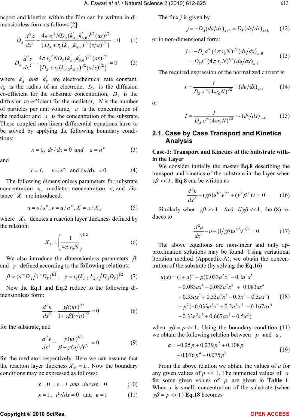 A. Eswari et al. / Natural Science 2 (2010) 612-625 Copyright © 2010 SciRes. OPEN ACCESS 613 613 nsport and kinetics within the film can be written in di- mensionless form as follows [2]: askkrD askkNDr dx ad D SAA SAA A0 ])()([ )()(4 2121' 0, ' 0,0 2121' 0, ' 0, 2 0 2 2 (1) 0 ])()([ )()(4 2121' 0, ' 0,0 2121' 0, ' 0, 2 0 2 2 sakkrD askkNDr dx sd D SAS SAS S (2) where '' SA k and k are electrochemical rate constant, 0 r is the radius of an electrode, S D is the diffusion co-efficient for the substrate concentration, A D is the diffusion co-efficient for the mediator, Nis the number of particles per unit volume, a is the concentration of the mediator and is the concentration of the substrate. These coupled non-linear differential equations have to be solved by applying the following boundary condi- tions: aa and xdsd x0/,0 (3) and , and d/d 0 xL ssax (4) The following dimensionless parameters for substrate concentration ,u mediator concentration ,vand dis- tance are introduced: K XxXaavssu /,/,/ (5) where k X denotes a reaction layer thickness defined by the relation: Nr Xk 2/1 0 4 1 (6) We also introduce the dimensionless parameters and defined according to the following relations: DsDaSA ,)( 21 21' 0, ' 0,0 )( SASA DDk kr (7) Now the Eq.1 and Eq.2 reduce to the following di- mensionless form: 0 )(1 )( 21 21 2 2 uv uv dx ud (8) for the substrate, and 0 )( )( 21 21 2 2 vu uv dx vd (9) for the mediator respectively. Here we can assume that the reaction layer thicknessLX K. Now the boundary conditions may be expressed as follows: xdud and 1v ,x0/0 (10) 1x, 0 xdvd and u1 (11) The flux j is given by jLxSxA xdsdDxdadD )()( 0 (12) or in non-dimensional form: xdudNr sD xdvdNr aDj xS xA 1 21 0 0 21 0 )()4( )()4( (13) The required expression of the normalized current is 21 0)4( Nrs D j I S =1 )(x xdud (14) or 21 0)4( Nra D j I A =- 0 )( x xdvd (15) 2.1. Case by Case Transport and Kinetics Analysis Case-1: Transport and Kinetics of the Substrate with- in the Layer We consider initially the master Eq.8 describing the transport and kinetics of the substrate in the layer when 1 . Eq.8 can be written as vvu dx ud 0)()( 222121 2 2 (16) Similarly when 11 1 (or) , the (8) re- duces to vuu dx ud 0)1( 2121 2 2 (17) The above equations are non-linear and only ap- proximation solutions may be found. Using variational iteration method (Appendix-A), we obtain the concen- tration of the substrate (by solving the Eq .16) 22625 4244 32322 22625 4 243 2 () (1)(0.0330.1 0.0830.083 0.083 0.330.330.50.5) (0.0330.2 0.167 0.33a0.6670.5) uxa paxax axa xax axa xxax paxax ax xaxx (18) when 1 p . Using the boundary condition (11) we obtain the following relation between p and a. 54 32 075.0076.0 108.0239.025.0 pp pppa (19) From the above relation we obtain the values of a for any given values of p << 1. The numerical values of a for some given values of p are given in Table 1. When x is small, concentration of the substrate (when 1 p ) Eq.18 becomes 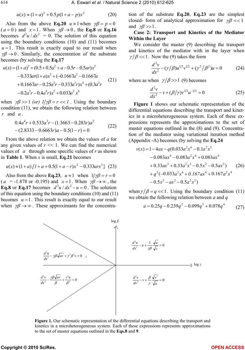 A. Eswari et al. / Natural Science 2 (2010) 612-625 Copyright © 2010 SciRes. OPEN ACCESS 614 22 )1(5.0)1()( xpapaxu (20) Also from the above Eq.20 1uwhen 0 p (0a) and 1x. When 0 , the Eq.8 or Eq.16 becomes ud 2/2 dx = 0. The solution of this equation using the boundary conditions (10) and (11) becomes 1u. This result is exactly equal to our result when 0 . Similarly, the concentration of the substrate becomes (by solving the Eq.17 62543 2432 23 222 033.0)4.02.0 3.0()333.025.01667.0 1667.01667.0()1(333.0 )5.05.05.05.0()1()( x axra ra raxraraar aa xaar xarraaaxu (21) when 1r1 (or) 1. Using the boundary condition (11), we obtain the following relation between and a. 0)1(5.0)6663.08333.2( )283.03663.1(533.04.0 234 rar arrara (22) From the above relation we obtain the values of a for any given values of r << 1. We can find the numerical values of a through some specific values of r as shown in Table 1. When x is small, Eq.21 becomes ]333.0)1(5.0)1()( 32 arxxraa[1 axu (23) Also from the above Eq.23, 1u when 01 r (a = -1.878 or -0.195) and 1 x. When , the Eq.8 or Eq.17 becomes ud2/0 2 udx. The solution of this equation using the boundary conditions (10) and (11) becomes 1u. This result is exactly equal to our result when . These approximants for the concentra- tion of the substrate Eq.20, Eq.23 are the simplest closed- form of analytical approximation for 1 and 1 . Case 2: Transport and Kinetics of the Mediator Within the Layer We consider the master (9) describing the transport and kinetics of the mediator with in the layer when . 1 Now the (9) takes the form 0)()( 222121 2 2 uvu dx vd (24) where as when 1 (9) becomes 0)( 2123 2 2 uvv dx vd (25) Figure 1 shows our schematic representation of the differential equations describing the transport and kinet- ics in a microheterogeneous system. Each of these ex- pressions represents the approximations to the set of master equations outlined in the (8) and (9). Concentra- tion of the mediator using variational iteration method (Appendix -A) becomes (by solving the Eq.24 xaaxx xaax0.167 xaq axxxaax axxaax xaxaqaxxv )5.05.0 167.0033.0( )5.05.033.033.0 083.0083.0083.0 1.0033.0(41)( 2222 424622 22323 4426 5262 (26) when 1 q . Using the boundary condition (11) we obtain the following relation between a and q 432 078.0099.0239.025.0 qqqqa (27) log β log γ 0 1 2 2 v u u dx ud 0 3 2 2 u v v dx vd 0 2 2 2 2 uuv dx vd 0 22 2 2 vuv dx ud Figure 1. Our schematic representation of the differential equations describing the transport and kinetics in a microheterogeneous system. Each of these expressions represents approximations to the set of master equations outlined in the Eqs.8 and 9. 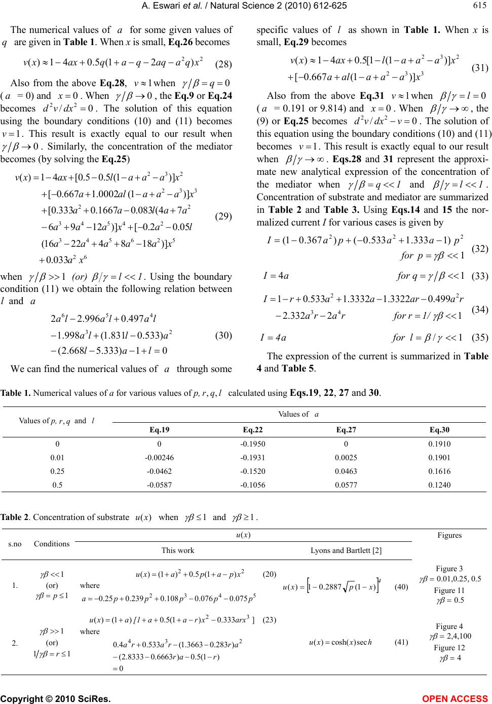 A. Eswari et al. / Natural Science 2 (2010) 612-625 Copyright © 2010 SciRes. OPEN ACCESS 615 615 The numerical values of a for some given values of q are given in Table 1. When x is small, Eq.26 becomes 22 )21(5.041)( xqaaqqaqaxxv (28) Also from the above Eq.28, 1vwhen 0 q (a = 0) and 0x. When 0 , the Eq.9 or Eq.24 becomes 0/ 22 dxvd . The solution of this equation using the boundary conditions (10) and (11) becomes 1v. This result is exactly equal to our result when 0 . Similarly, the concentration of the mediator becomes (by solving the Eq.25) 62 526543 24543 22 332 232 033.0 )]18842216( 05.02.0[)]1296 74(083.01667.0333.0[ )]1(0002.1667.0[ )]1(5.05.0[41)( x a xaaaaa laxaaa aalaa xaaa ala xaaalaxxv (29) when 1l (or) 1. Using the boundary condition (11) we obtain the following relation between and a lal alla lalala 01)333.5668.2( )533.0831.1(998.1 497.0996.22 23 456 (30) We can find the numerical values of a through some specific values of l as shown in Table 1. When x is small, Eq.29 becomes 332 232 )]1(667.0[ )]1(1[5.041)( xaaaala xaaalaxxv (31) Also from the above Eq.31 1vwhen 0 l (a = 0.191 or 9.814) and 0x. When , the (9) or Eq.25 becomes 0/ 22 vdxvd . The solution of this equation using the boundary conditions (10) and (11) becomes 1 v. This result is exactly equal to our result when . Eqs.28 and 31 represent the approxi- mate new analytical expression of the concentration of the mediator when 1q and 1l . Concentration of substrate and mediator are summarized in Table 2 and Table 3. Using Eqs.14 and 15 the nor- malized current I for various cases is given by 1 )1333.1533.0()367.01( 222 p for p aapaI (32) 14 q for aI (33) 1/r for rara raaraarI 12332.2 499.03322.13332.1533.01 43 22 (34) l for a4I1/ (35) The expression of the current is summarized in Table 4 and Table 5. Table 1. Numerical values of a for various values of p, l q r,, calculated using Eqs.19, 22, 27 and 30. Values of a Values of p, q ,and l Eq.19 Eq.22 Eq.27 Eq.30 0 0 -0.1950 0 0.1910 0.01 -0.00246 -0.1931 0.0025 0.1901 0.25 -0.0462 -0.1520 0.0463 0.1616 0.5 -0.0587 -0.1056 0.0577 0.1240 Table 2. Concentration of substrate )(xu when 1 and 1 . )( xu Figures s.no Conditions This work Lyons and Bartlett [2] 1. 1 (or) 1 p 22 )1(5.0)1()( xpapaxu (20) where 5432 075.0076.0108.0239.025.0pppppa xpxu4 )1(2887.01)( (40) Figure 3 0.01,0.25, 0.5 Figure 11 0.5 2. 1 (or) 11 r 32 333.0)1(5.0)1()( arxxraa[1 axu] (23) where 0 )1(5.0)6663.08333.2( )283.03663.1(533.04.0 234 rar arrara hxxu sec)cosh()( (41) Figure 4 2,4,100 Figure 12 4 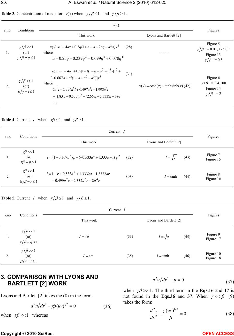 A. Eswari et al. / Natural Science 2 (2010) 612-625 Copyright © 2010 SciRes. OPEN ACCESS 616 Table 3. Concentration of mediator )(xv when 1 and 1 . )(xv s.no Conditions This work Lyons and Bartlett [2] Figures 1. 1 (or) 1q 22 )21(5.041)( xqaaqqaqaxxv (28) where 432 078.0099.0239.025.0 qqqqa -------- Figure 5 = 0.01,0.25,0.5 Figure 13 = 0.5 2. 1 (or) 1 l 332 232 )]1(667.0[ )]1(1[5.041)( xaaaala xaaalaxxv (31) where lalal lalalala 0 1)333.5668.2()533.0831.1( 998.1497.0996.22 2 3456 )sinh(tanh)cosh()( xxxv (42) Figure 6 = 2,4,100 Figure 14 = 2 Table 4. Current when 1 and 1 . Current I s.no Conditions This work Lyons and Bartlett [2] Figures 1. 1 (or) 1 p p aapaI222 )1333.1533.0()367.01( (32)pI (43) Figure 7 Figure 15 2. 1 (or) 11 r rarara araarI 432 2 2332.2499.0 3322.13332.1533.01 (34)tanh I (44) Figure 8 Figure 16 Table 5. Current when 1 and 1 . Current I s.no Conditions This work Lyons and Bartlett [2] Figures 1. 1 (or) 1q aI4 (33)qI (45) Figure 9 Figure 17 2. 1 (or) 1l aI4 (35)tanhI (46) Figure 10 Figure 18 3. COMPARISON WITH LYONS AND BARTLETT [2] WORK Lyons and Bartlett [2] takes the (8) in the form 0)( 2122 uvdxud (36) when 1 whereas 0 22 udxud (37) when 1 . The third term in the Eqs.16 and 17 is not found in the Eqs.36 and 37. When (9) takes the form: 0 )( 21 2 2 uv dx vd (38) 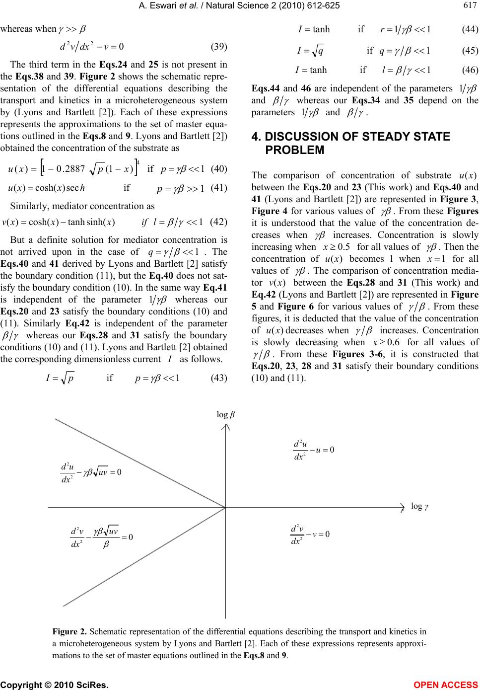 A. Eswari et al. / Natural Science 2 (2010) 612-625 Copyright © 2010 SciRes. OPEN ACCESS 617 617 whereas when 0 22 vdxvd (39) The third term in the Eqs.24 and 25 is not present in the Eqs.38 and 39. Figure 2 shows the schematic repre- sentation of the differential equations describing the transport and kinetics in a microheterogeneous system by (Lyons and Bartlett [2]). Each of these expressions represents the approximations to the set of master equa- tions outlined in the Eqs.8 and 9. Lyons and Bartlett [2]) obtained the concentration of the substrate as 4 )1(2887.01)(xpxu if 1 p (40) hxxusec)cosh()( if 1 p (41) Similarly, mediator concentration as 1)sinh(tanh)cosh()( l if xxxv (42) But a definite solution for mediator concentration is not arrived upon in the case of q 1 . The Eqs.40 and 41 derived by Lyons and Bartlett [2] satisfy the boundary condition (11), but the Eq.40 does not sat- isfy the boundary condition (10). In the same way Eq.41 is independent of the parameter 1 whereas our Eqs.20 and 23 satisfy the boundary conditions (10) and (11). Similarly Eq.42 is independent of the parameter whereas our Eqs.28 and 31 satisfy the boundary conditions (10) and (11). Lyons and Bartlett [2] obtained the corresponding dimensionless current as follows. pI if 1 p (43) tanh I if 11 r (44) qI if 1 q (45) tanh I if 1 l (46) Eqs.44 and 46 are independent of the parameters 1 and whereas our Eqs.34 and 35 depend on the parameters 1 and . 4. DISCUSSION OF STEADY STATE PROBLEM The comparison of concentration of substrate )(xu between the Eqs.20 and 23 (This work) and Eqs.40 and 41 (Lyons and Bartlett [2]) are represented in Figure 3, Figure 4 for various values of . From these Figures it is understood that the value of the concentration de- creases when increases. Concentration is slowly increasing when 5.0x for all values of . Then the concentration of )(xu becomes 1 when 1 x for all values of . The comparison of concentration media- tor )(xv between the Eqs.28 and 31 (This work) and Eq.42 (Lyons and Bartlett [2]) are represented in Figure 5 and Figure 6 for various values of . From these figures, it is deducted that the value of the concentration of )(xudecreases when increases. Concentration is slowly decreasing when 6.0x for all values of . From these Figures 3-6, it is constructed that Eqs.20, 23, 28 and 31 satisfy their boundary conditions (10) and (11). log β log γ 0 2 2 u dx ud 0 2 2 v dx vd 0 2 2 uv dx vd 0 2 2 uv dx ud Figure 2. Schematic representation of the differential equations describing the transport and kinetics in a microheterogeneous system by Lyons and Bartlett [2]. Each of these expressions represents approxi- mations to the set of master equations outlined in the Eqs.8 and 9. 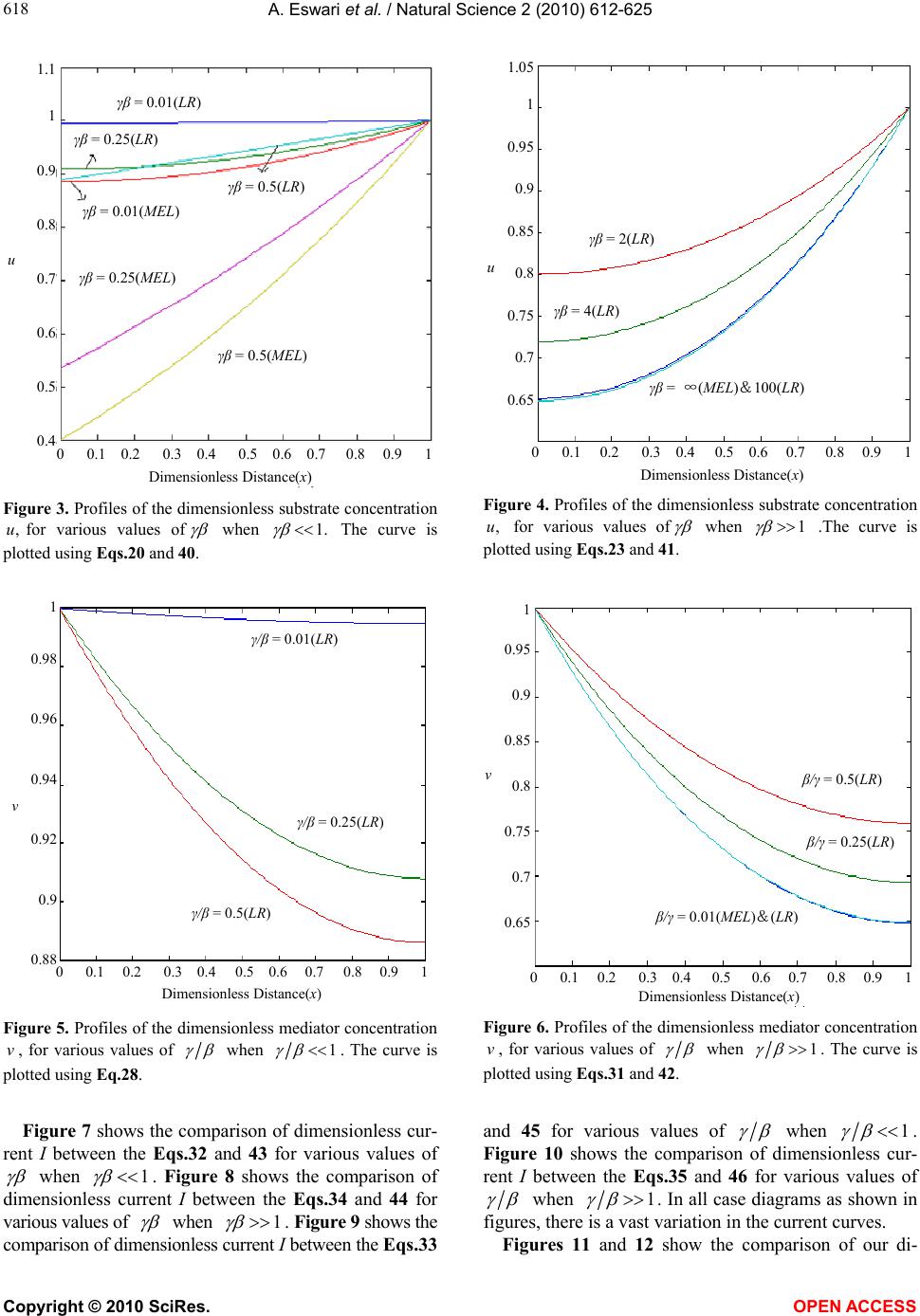 A. Eswari et al. / Natural Science 2 (2010) 612-625 Copyright © 2010 SciRes. OPEN ACCESS 618 Dimensionless Distance(x) u 0 0.1 0.2 0.3 0.4 0.5 0.6 0.7 0.8 0.9 1 1.1 1 0.9 0.8 0.7 0.6 0.5 0.4 γβ = 0.01(LR ) γβ = 0.25(LR) γβ = 0.5(LR) γβ = 0.5(MEL) γβ = 0.25(MEL) γβ = 0.01(MEL) Figure 3. Profiles of the dimensionless substrate concentration ,ufor various values of when .1 The curve is plotted using Eqs.20 and 40. Dimensionless Distance(x) u 0 0.1 0.2 0.3 0.4 0.5 0.6 0.7 0.8 0.9 1 1.05 1 0.95 0.9 0.85 0.8 0.75 0.7 0.65 γβ = 2(LR) γβ = 4(LR) γβ = ∞(MEL)&100(LR) Figure 4. Profiles of the dimensionless substrate concentration ,u for various values of when 1 .The curve is plotted using Eqs.23 and 41. Dimensionless Distance(x) v 1 0.98 0.96 0.94 0.92 0.9 0.88 γ/β = 0.01(LR) γ/β = 0.5(LR) γ/β = 0.25(LR) 0 0.1 0.2 0.3 0.4 0.5 0.6 0.7 0.8 0.9 1 Figure 5. Profiles of the dimensionless mediator concentration v, for various values of when 1 . The curve is plotted using Eq.28. vβ/γ = 0.5(LR) 0 0.1 0.2 0.3 0.4 0.5 0.6 0.7 0.8 0.9 1 β/γ = 0.25(LR) β/γ = 0.01(MEL)&(LR) 1 0.95 0.9 0.85 0.8 0.75 0.7 0.65 Dimensionless Distance(x) Figure 6. Profiles of the dimensionless mediator concentration v, for various values of when 1 . The curve is plotted using Eqs.31 and 42. Figure 7 shows the comparison of dimensionless cur- rent I between the Eqs.32 and 43 for various values of when 1 . Figure 8 shows the comparison of dimensionless current I between the Eqs.34 and 44 for various values of when 1 . Figure 9 shows the comparison of dimensionless current I between the Eqs.33 and 45 for various values of when 1 . Figure 10 shows the comparison of dimensionless cur- rent I between the Eqs.35 and 46 for various values of when 1 . In all case diagrams as shown in figures, there is a vast variation in the current curves. Figures 11 and 12 show the comparison of our di-  A. Eswari et al. / Natural Science 2 (2010) 612-625 Copyright © 2010 SciRes. OPEN ACCESS 619 619 mensionless concentration u evaluated using Eqs.20 and 23 (This work) together with the simulation results (This work) and Eqs.40 and 41 (Lyons and Bartlett [2]) for the case of 1 and 1 . Figures 13 and 14 indicate the comparison of our dimensionless con- centration v calculated using Eqs.28 and 31 (This work) together with the simulation results (This work) and Eq.42 (Lyons and Bartlett [2]) for the case of 1 and 1 . In all cases, there is a good match be- tween our analytical and simulation results. Figures 15 and 16 show the comparison of our di- mensionless current I versus evaluated using Eqs.32 and 34 (This work) together with the simulation results (This work) and Eqs.43 and 44 (Lyons and Bartlett [2]) for the case of 1 and 1 . Figures 17 and 18 indicate the comparison of our dimensionless current I versus calculated using Eqs.33 and 35 (This work) together with the simulation results (This work) and Eqs.45 and 46 (Lyons and Bartlett [2]) for the case of 1 and 1 . In all cases, there is a good Dimensionless current I γβ = p 0.9 0.8 0.7 0.6 0.5 0.4 0.3 0.2 0.1 0 -0.1 (30)-(LR) (41)-(MEL) 0 0.1 0.2 0.3 0.4 0.5 0.6 0.7 0.8 Figure 7. Plot of dimensionless current versus p . Cur- rent is calculated in the Eqs.32 and 43. Dimensionless current I 0.8 0.7 0.6 0.5 0.4 0.3 0.2 0.1 0 (32)-(LR) (42)-(MEL) 0 0.1 0.2 0.3 0.4 0.5 0.6 0.7 0.8 0.9 1 1/γβ = r Figure 8. Plot of dimensionless current versus r 1. Cur- rent is calculated in the Eqs.34 and 44. Dimensionless current I 1.2 1 0.8 0.6 0.4 0.2 0 -0.2 (31)-(LR) (43)-(MEL) 0 0.1 0.2 0.3 0.4 0.5 0.6 0.7 0.8 0.9 1 γ/β = q Figure 9. Plot of dimensionless current versus q . Cur- rent is calculated in the Eqs.33 and 45. Dimensionless current I 0.8 0.7 0.6 0.5 0.4 0.3 0.2 0.1 0 (33)-(LR) (44 ) -( MEL) 0 0.1 0.2 0.3 0.4 0.5 0.6 0.7 0.8 0.9 1 β/γ = l Figure 10. Plot of dimensionless current versus l . Cur- rent is calculated in the Eqs.35 and 46. 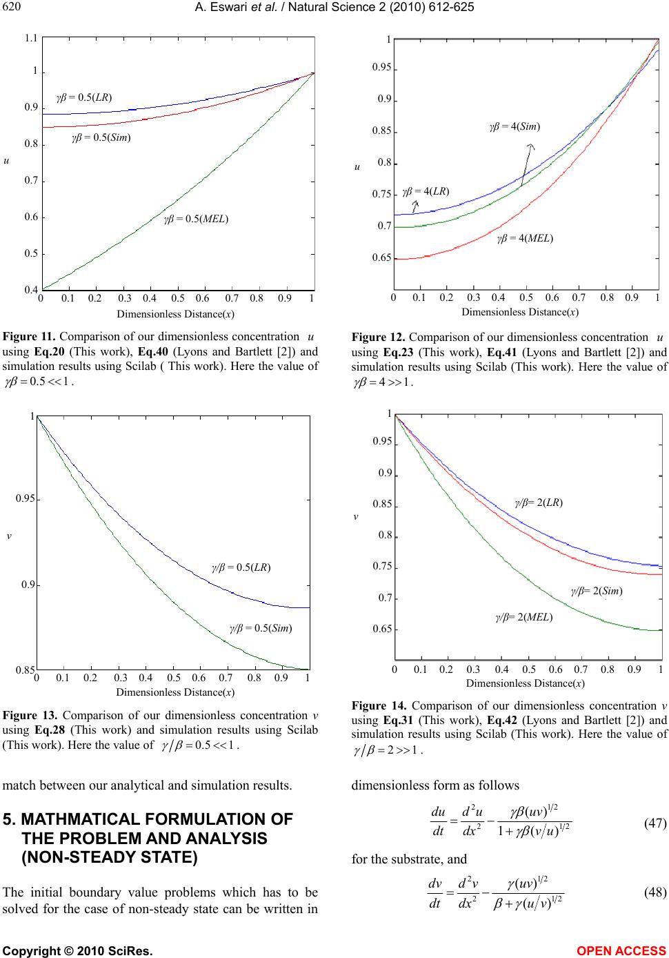 A. Eswari et al. / Natural Science 2 (2010) 612-625 Copyright © 2010 SciRes. OPEN ACCESS 620 u 0 0.1 0.2 0.3 0.4 0.5 0.6 0.7 0.8 0.9 1 1.1 1 0.9 0.8 0.7 0.6 0.5 0.4 γβ = 0.5(LR) γβ = 0.5(MEL) γβ = 0.5(Sim) Dimensionless Distance(x) Figure 11. Comparison of our dimensionless concentration u using Eq.20 (This work), Eq.40 (Lyons and Bartlett [2]) and simulation results using Scilab ( This work). Here the value of 15.0 . Dimensionless Distance(x) u 0 0.1 0.2 0.3 0.4 0.5 0.6 0.7 0.8 0.9 1 1 0.95 0.9 0.85 0.8 0.75 0.7 0.65 γβ = 4(MEL) γβ = 4(LR) γβ = 4(Sim) Figure 12. Comparison of our dimensionless concentration u using Eq.23 (This work), Eq.41 (Lyons and Bartlett [2]) and simulation results using Scilab (This work). Here the value of 14 . v 1 0.95 0.9 0.85 γ/β = 0.5(LR) 0 0.1 0.2 0.3 0.4 0.5 0.6 0.7 0.8 0.9 1 γ/β = 0.5(Sim) Dimensionless Distance(x) Figure 13. Comparison of our dimensionless concentration v using Eq.28 (This work) and simulation results using Scilab (This work). Here the value of 15.0 . v 0 0.1 0.2 0.3 0.4 0.5 0.6 0.7 0.8 0.9 1 γ/β= 2(LR) 1 0.95 0.9 0.85 0.8 0.75 0.7 0.65 γ/β= 2(Sim) γ/β= 2(MEL) Dimensionless Distance(x) Figure 14. Comparison of our dimensionless concentration v using Eq.31 (This work), Eq.42 (Lyons and Bartlett [2]) and simulation results using Scilab (This work). Here the value of 12 . match between our analytical and simulation results. 5. MATHMATICAL FORMULATION OF THE PROBLEM AND ANALYSIS (NON-STEADY STATE) The initial boundary value problems which has to be solved for the case of non-steady state can be written in dimensionless form as follows 21 21 2 2 )(1 )( uv uv dx ud dt du (47) for the substrate, and vu uv dx vd dt dv 21 21 2 2 )( )( (48) 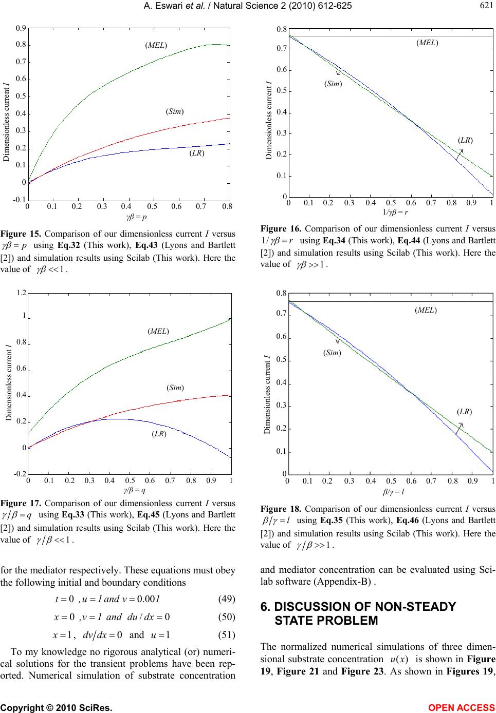 A. Eswari et al. / Natural Science 2 (2010) 612-625 Copyright © 2010 SciRes. OPEN ACCESS 621 621 γβ = p 0.9 0.8 0.7 0.6 0.5 0.4 0.3 0.2 0.1 0 -0.1 (MEL) (Sim) 0 0.1 0.2 0.3 0.4 0.5 0.6 0.7 0.8 (LR) Dimensionless current I Figure 15. Comparison of our dimensionless current I versus p using Eq.32 (This work), Eq.43 (Lyons and Bartlett [2]) and simulation results using Scilab (This work). Here the value of 1 . Dimensionless current I 0.8 0.7 0.6 0.5 0.4 0.3 0.2 0.1 0 (LR) (MEL) 0 0.1 0.2 0.3 0.4 0.5 0.6 0.7 0.8 0.9 1 1/γβ = r (Sim) Figure 16. Comparison of our dimensionless current I versus r /1 using Eq.34 (This work), Eq.44 (Lyons and Bartlett [2]) and simulation results using Scilab (This work). Here the value of 1 . Dimensionless current I 1.2 1 0.8 0.6 0.4 0.2 0 -0.2 (LR) (MEL) 0 0.1 0.2 0.3 0.4 0.5 0.6 0.7 0.8 0.9 1 γ/β = q (Sim) Figure 17. Comparison of our dimensionless current I versus q using Eq.33 (This work), Eq.45 (Lyons and Bartlett [2]) and simulation results using Scilab (This work). Here the value of 1 . Dimensionless current I 0.8 0.7 0.6 0.5 0.4 0.3 0.2 0.1 0 (LR) (MEL) 0 0.1 0.2 0.3 0.4 0.5 0.6 0.7 0.8 0.9 1 β/γ = l (Sim) Figure 18. Comparison of our dimensionless current I versus l using Eq.35 (This work), Eq.46 (Lyons and Bartlett [2]) and simulation results using Scilab (This work). Here the value of 1 . for the mediator respectively. These equations must obey the following initial and boundary conditions 1v and 1u ,t00.00 (49) 0/0 dxdu and 1v ,x (50) 1x, 0dxdv and u1 (51) To my knowledge no rigorous analytical (or) numeri- cal solutions for the transient problems have been rep- orted. Numerical simulation of substrate concentration and mediator concentration can be evaluated using Sci- lab software (Appendix-B) . 6. DISCUSSION OF NON-STEADY STATE PROBLEM The normalized numerical simulations of three dimen- sional substrate concentration )(xu is shown in Figure 19, Figure 21 and Figure 23. As shown in Figures 19, 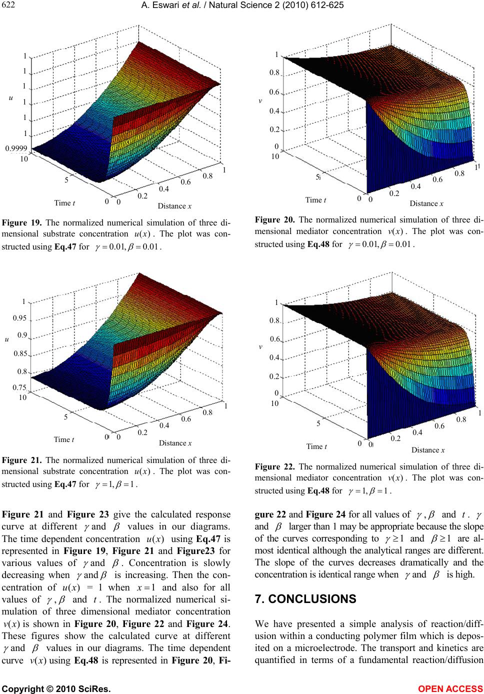 A. Eswari et al. / Natural Science 2 (2010) 612-625 Copyright © 2010 SciRes. OPEN ACCESS 622 u 1 Time t Distance x 0.8 0.6 0.4 0.2 0 0 5 10 0.9999 1 1 1 1 1 1 Figure 19. The normalized numerical simulation of three di- mensional substrate concentration )(xu. The plot was con- structed using Eq.47 for 01.0,01.0 . v 1 Time tDistance x 0.8 0.6 0.4 0.2 0 0 5 10 1 0 0.2 0.4 0.6 0.8 Figure 20. The normalized numerical simulation of three di- mensional mediator concentration )(xv . The plot was con- structed using Eq.48 for 01.0,01.0 . u 1 Time t Distance x 0.8 0.6 0.4 0.2 0 0 5 10 1 0.95 0.9 0.85 0.8 0.75 Figure 21. The normalized numerical simulation of three di- mensional substrate concentration )(xu. The plot was con- structed using Eq.47 for 1,1 . v 1 Time tDistance x 0.8 0.6 0.4 0.2 0 0 5 10 1 0.8 0.6 0.4 0.2 0 Figure 22. The normalized numerical simulation of three di- mensional mediator concentration )(xv . The plot was con- structed using Eq.48 for 1,1 . Figure 21 and Figure 23 give the calculated response curve at different and values in our diagrams. The time dependent concentration )(xu using Eq.47 is represented in Figure 19, Figure 21 and Figure23 for various values of and . Concentration is slowly decreasing when and is increasing. Then the con- centration of )(xu = 1 when 1x and also for all values of , and . The normalized numerical si- mulation of three dimensional mediator concentration )(xv is shown in Figure 20, Figure 22 and Figure 24. These figures show the calculated curve at different and values in our diagrams. The time dependent curve )(xv using Eq.48 is represented in Figure 20, Fi- gure 22 and Figure 24 for all values of , and . and larger than 1 may be appropriate because the slope of the curves corresponding to 1 and 1 are al- most identical although the analytical ranges are different. The slope of the curves decreases dramatically and the concentration is identical range when and is high. 7. CONCLUSIONS We have presented a simple analysis of reaction/diff- usion within a conducting polymer film which is depos- ited on a microelectrode. The transport and kinetics are quantified in terms of a fundamental reaction/diffusion 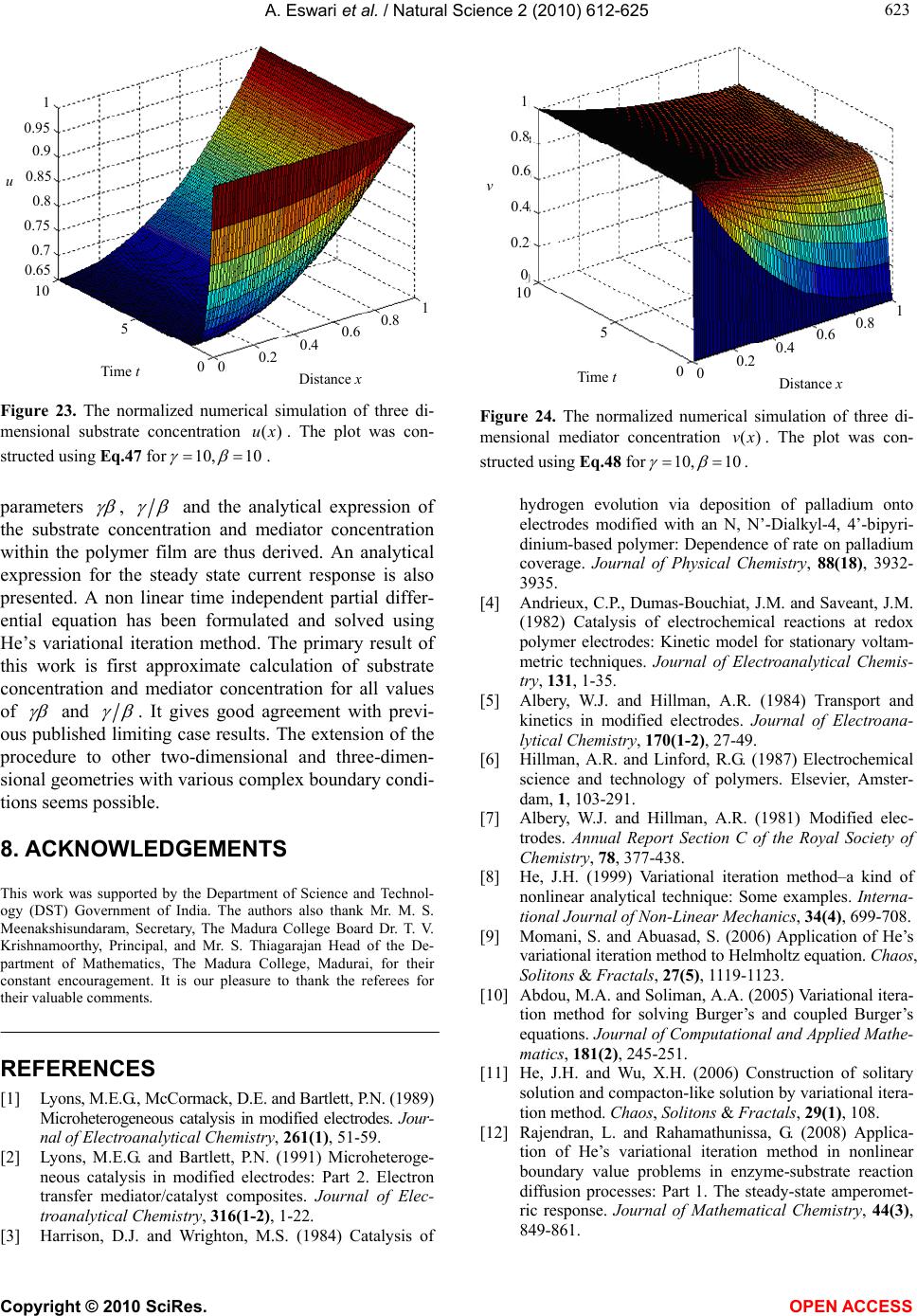 A. Eswari et al. / Natural Science 2 (2010) 612-625 Copyright © 2010 SciRes. OPEN ACCESS 623 623 u 1 Time t Distance x 0.8 0.6 0.4 0.2 0 0 5 10 1 0.95 0.9 0.85 0.8 0.75 0.7 0.65 Figure 23. The normalized numerical simulation of three di- mensional substrate concentration )(xu. The plot was con- structed using Eq.47 for10,10 . v 1 Time tDistance x 0.8 0.6 0.4 0.2 0 0 5 10 1 0.8 0.6 0.4 0.2 0 Figure 24. The normalized numerical simulation of three di- mensional mediator concentration )(xv . The plot was con- structed using Eq.48 for10,10 . parameters , and the analytical expression of the substrate concentration and mediator concentration within the polymer film are thus derived. An analytical expression for the steady state current response is also presented. A non linear time independent partial differ- ential equation has been formulated and solved using He’s variational iteration method. The primary result of this work is first approximate calculation of substrate concentration and mediator concentration for all values of and . It gives good agreement with previ- ous published limiting case results. The extension of the procedure to other two-dimensional and three-dimen- sional geometries with various complex boundary condi- tions seems possible. 8. ACKNOWLEDGEMENTS This work was supported by the Department of Science and Technol- ogy (DST) Government of India. The authors also thank Mr. M. S. Meenakshisundaram, Secretary, The Madura College Board Dr. T. V. Krishnamoorthy, Principal, and Mr. S. Thiagarajan Head of the De- partment of Mathematics, The Madura College, Madurai, for their constant encouragement. It is our pleasure to thank the referees for their valuable comments. REFERENCES [1] Lyons, M.E.G., McCormack, D.E. and Bartlett, P.N. (1989) Microheterogeneous catalysis in modified electrodes. Jour- nal of Electroanalytical Chemistry, 261(1), 51-59. [2] Lyons, M.E.G. and Bartlett, P.N. (1991) Microheteroge- neous catalysis in modified electrodes: Part 2. Electron transfer mediator/catalyst composites. Journal of Elec- troanalytical Chemistry, 316(1-2), 1-22. [3] Harrison, D.J. and Wrighton, M.S. (1984) Catalysis of hydrogen evolution via deposition of palladium onto electrodes modified with an N, N’-Dialkyl-4, 4’-bipyri- dinium-based polymer: Dependence of rate on palladium coverage. Journal of Physical Chemistry, 88(18), 3932- 3935. [4] Andrieux, C.P., Dumas-Bouchiat, J.M. and Saveant, J.M. (1982) Catalysis of electrochemical reactions at redox polymer electrodes: Kinetic model for stationary voltam- metric techniques. Journal of Electroanalytical Chemis- try, 131, 1-35. [5] Albery, W.J. and Hillman, A.R. (1984) Transport and kinetics in modified electrodes. Journal of Electroana- lytical Chemistry, 170(1-2), 27-49. [6] Hillman, A.R. and Linford, R.G. (1987) Electrochemical science and technology of polymers. Elsevier, Amster- dam, 1, 103-291. [7] Albery, W.J. and Hillman, A.R. (1981) Modified elec- trodes. Annual Report Section C of the Royal Society of Chemistry, 78, 377-438. [8] He, J.H. (1999) Variational iteration method–a kind of nonlinear analytical technique: Some examples. Interna- tional Journal of Non-Linear Mechanics, 34(4), 699-708. [9] Momani, S. and Abuasad, S. (2006) Application of He’s variational iteration method to Helmholtz equation. Chaos, Solitons & Fractals, 27(5), 1119-1123. [10] Abdou, M.A. and Soliman, A.A. (2005) Variational itera- tion method for solving Burger’s and coupled Burger’s equations. Journal of Computational and Applied Mathe- matics, 181(2), 245-251. [11] He, J.H. and Wu, X.H. (2006) Construction of solitary solution and compacton-like solution by variational itera- tion method. Chaos, Solitons & Fractals, 29(1), 108. [12] Rajendran, L. and Rahamathunissa, G. (2008) Applica- tion of He’s variational iteration method in nonlinear boundary value problems in enzyme-substrate reaction diffusion processes: Part 1. The steady-state amperomet- ric response. Journal of Mathematical Chemistry, 44(3), 849-861. 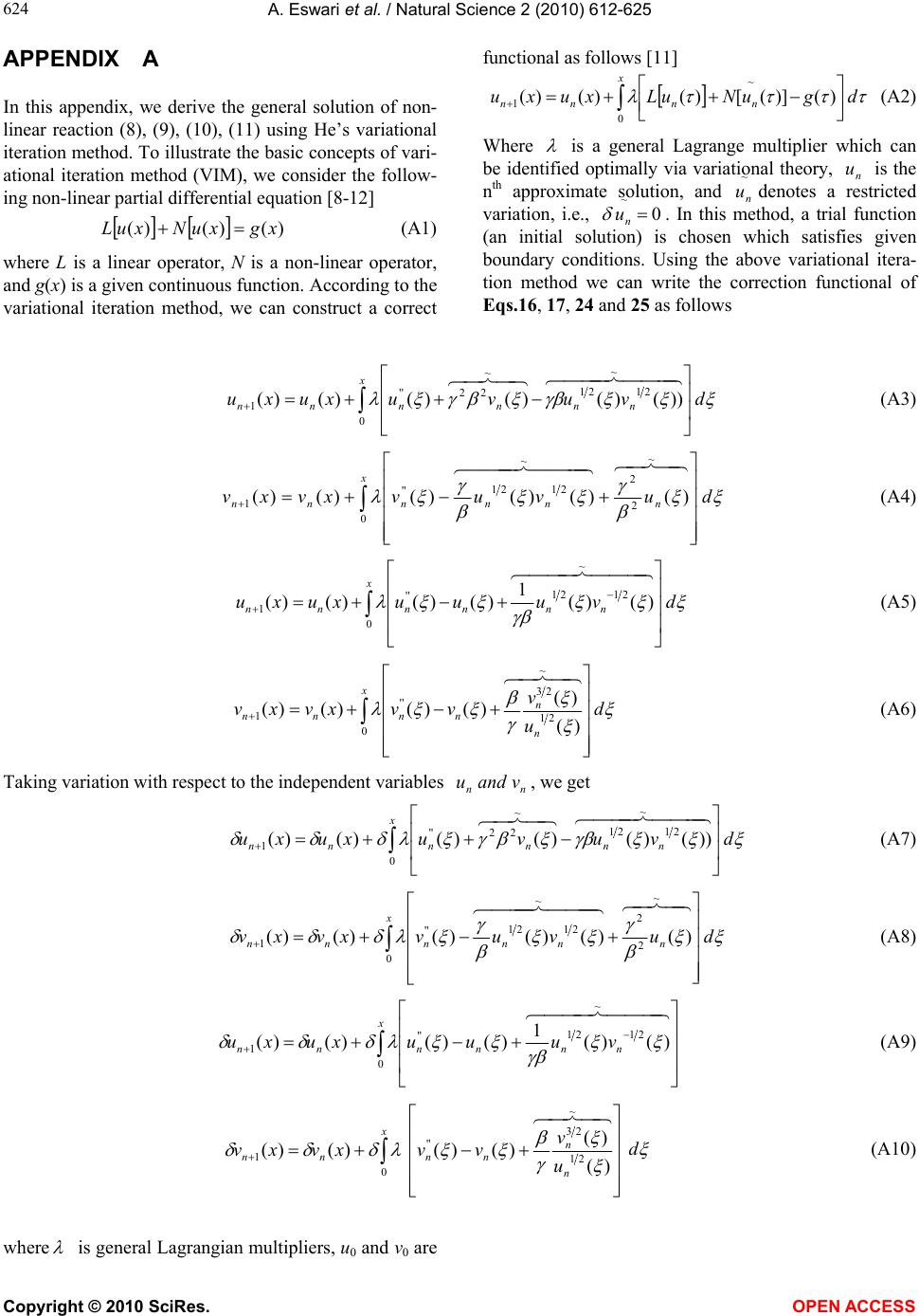 A. Eswari et al. / Natural Science 2 (2010) 612-625 Copyright © 2010 SciRes. OPEN ACCESS 624 APPENDIX A In this appendix, we derive the general solution of non- linear reaction (8), (9), (10), (11) using He’s variational iteration method. To illustrate the basic concepts of vari- ational iteration method (VIM), we consider the follow- ing non-linear partial differential equation [8-12] )()()(xgxuNxuL (A1) where L is a linear operator, N is a non-linear operator, and g(x) is a given continuous function. According to the variational iteration method, we can construct a correct functional as follows [11] d guNuLxuxu x nnnn 0 ~ 1)()]([)()()( (A2) Where is a general Lagrange multiplier which can be identified optimally via variational theory, n u is the nth approximate solution, and ~ n udenotes a restricted variation, i.e., 0 ~ n u . In this method, a trial function (an initial solution) is chosen which satisfies given boundary conditions. Using the above variational itera- tion method we can write the correction functional of Eqs.16, 17, 24 and 25 as follows d vuvuxuxu x nnnnnn 0 ~ 2121 ~ 22'' 1))()()()()()( (A3) d uvuvxvxv x nnnnnn 0 ~ 2 2 ~ 2121 '' 1)()()()()()( (A4) d vuuuxuxu x nnnnnn 0 ~ 2121 '' 1)()( 1 )()()()( (A5) d u v vvxvxv x n n nnnn 0 ~ 21 23 '' 1)( )( )()()()( (A6) Taking variation with respect to the independent variables nn v and u, we get d vuvuxuxunnnn x nn ~ 2121 ~ 22'' 0 1))()()()()()( (A7) d uvuvxvxvnnnn x nn ~ 2 2 ~ 2121 '' 0 1)()()()()()( (A8) x nnnnnn vuuuxuxu 0 ~ 2121 '' 1)()( 1 )()()()( (A9) x nn xvxv 0 1)()( ~ 21 23 '' )( )( )()( n n nn u v vv d (A10) where is general Lagrangian multipliers, u0 and v0 are  A. Eswari et al. / Natural Science 2 (2010) 612-625 Copyright © 2010 SciRes. OPEN ACCESS 625 625 initial approximations or trial functions ,vn ~ 22 )( ~ 2121 ))()( nn vu , ~ 2121)()( nn vu , ~ 2 2 )( n u ~ 2121 )()( 1 nnvu , ~ 21 23 )( )( n n u v and are considered as restricted variations i.e. 0 0 nn v ,u and 0 nnvu . Making the above correction functional (A7) to (A10) stationary, noticing that 0)0(0)0( nn v ,u and 0)0()0( nn v u . 0:' x n)(-1 u ,0 ' )(- 1:vn (A11) u n: ' 0)( x , 0)(: ' x n v (A12) 0)(: '' x n u , 0)(: '' x n v (A13) The above equations are called Lagrange-Euler equa- tions. By solving the above equations the Lagrange mul- tipliers, can be identified as )()(x (A14) substituting the Lagrangian multipliers and n = 0 in the iteration formula (A3, A4, A5, A6) we obtain, dvvuuxxuxu )]()()()([)()()( 0 2221 0 21 0 '' 0 0 01 (A15) dvuuuxxuxu )]()()1()()([)()()( 21 0 21 00 '' 0 0 01 (A16) duvuvxxvxv ])()()()()()[()()( 0 0 2221 0 21 0 '' 001 (A17) duvvvxxvxv ])()()()()()[()()( 0 21 0 23 00 '' 001 (A18) Assuming that its initial approximate solutions which satisfies the boundary conditions (10), (11) have the form xaxu22 0)]1(1[)( (A19) 22 0]21[)( axaxxv (A20) By the iteration formula (A15) to (A18) we have the Eqs.18, 21, 26 and 29 in the text. APPENDIX B Scilab Program to find a solution of the Eqs.47 -51. function pdex4 m = 0; x = linspace(0,1); t=linspace(0,1); sol = pdepe(m,@pdex4pde,@pdex4ic,@pdex4bc,x,t); u1 = sol(:,:,1); u2 = sol(:,:,2); figure surf(x,t,u1) title('u1(x,t)') xlabel('Distance x') ylabel('Time t') figure surf(x,t,u2) title('u2(x,t)') xlabel('Distance x') ylabel('Time t') % -------------------------------------------------------------- function [c,f,s] = pdex4pde(x,t,u,DuDx) c = [1; 1]; f = [1; 1] .* DuDx; y = u(1) * u(2); gamma=0.01; beta=0.01; % parameters F =(gamma*beta*sqrt(y))/(1+gamma*beta*(sqrt(u(2)/ u(1)))); F1=(gamma*sqrt(y))/( beta+gamma*(sqrt(u(1)/u(2)))); % non linear terms s=[-F;-F1]; % -------------------------------------------------------------- function u0 = pdex4ic(x); %create a initial conditions u0 = [1; 0.001]; % -------------------------------------------------------------- function [pl,ql,pr,qr] = pdex4bc(xl,ul,xr,ur,t) %create a boundary conditions pl = [0; ul(2)-1]; ql = [1; 0]; pr = [ur(1)-1; 0]; qr = [0; 1];
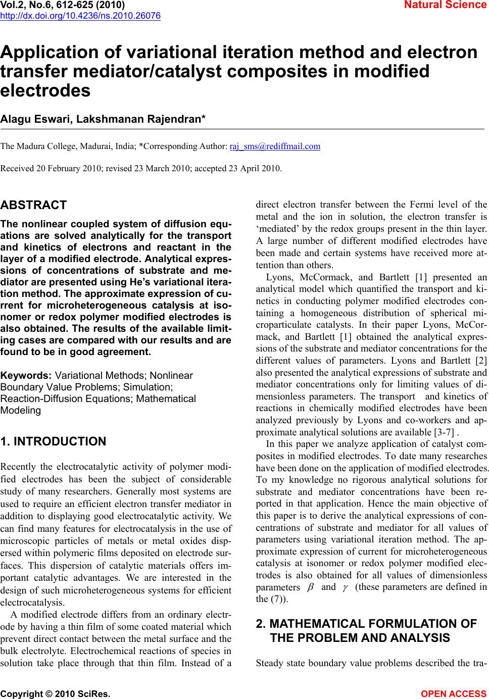
|