Vol.2, No.6, 576-589 (2010) Natural Science
http://dx.doi.org/10.4236/ns.2010.26073
Building reliable genetic maps: different mapping
strategies may result in different maps
Yefim Ronin, David Mester, Dina Minkov, Abraham Korol*
Institute of Evolution and Department of Evolutionary and Environmental Biology University of Haifa, Mount Carmel, Haifa, Israel;
*Corresponding Author:
Received 24 November 2009; revised 4 January 2010; accepted 6 April 2010.
ABSTRACT
New high throughput DNA technologies resul-
ted in a disproportion between the high number
of scored markers for the mapping populations
and relatively small sizes of the genotyped pop-
ulations. Correspondingly, the number of mark-
ers may, by orders of magnitude, exceed the
threshold of recombination resolution achieva-
ble for a given population size. Hence, only a
small part of markers can be genuinely ordered
in the map. The question is how to choose the
most informative markers for building such a
reliable “skeleton” map. We believe that our ap-
proach provides a solution to this difficult pro-
blem due to: 1) powerful tools of discrete opti-
mization for multilocus ordering; 2) a verifica-
tion procedure, which is impossible without fast
and high-quality optimization, to control the map
quality based on re-sampling techniques; 3) an
interactive algorithm of marker clustering in co-
mplicated situations caused by significant de-
viation of recombination rates between markers
of non-homologous chromosomes from the ex-
pected 50% (referred to as quasi-linkage or pse-
udo-linkage); and 4) an algorithm for detection
and removing excessive markers to increase
the stability of multilocus ordering.
Keywords: Pseudo-Linkage; Skeleton Map; Map
Verification; Map Stability; Traveling Salesperson
Problem; Guided Evolution Strategy
1. INTRODUCTION
Genetic maps are an important tool in genomics and in
numerous practical applications such as breeding, medi-
cal genetics, and gene cloning. Unfortunately, the avail-
able algorithms and software tools become less suitable
with an increasing number of available markers. The
objective of our study is to develop efficient methodol-
ogy for building multilocus genetic maps, providing the
control of the quality of maps by detecting and removing
the sources of map instability. Two major problems
should be addressed in multilocus genetic mapping: 1)
markers that belong to non-homologous chromosomes
should not be assigned to the same linkage group; and 2)
markers from the same chromosome should be placed on
the genetic map in the same order as the corresponding
DNA sequences that reside in the chromosome.
In situations with significant deviations of the recom-
bination rates between non-synthetic markers from the
expected level (50%), the problem of correct clustering
cannot be solved by an arbitrary choice of a certain
(constant) threshold value of recombination or LOD,
albeit this is exactly how this problem is treated in many
mapping packages [1,2]. Indeed, in experiments with the
foregoing characteristics, the recombination values be-
tween groups of markers from different chromosomes
may sometimes be smaller than the values between ad-
jacent markers within a chromosome. This phenomenon,
referred to as “quasi-linkage” (or “pseudo-linkage”) can
result from a combination of statistical and biological
reasons and scoring errors. The statistical reasonsof
pseudo-linkage are mainly caused by the sample size and
number of chromosomes (n) in the genome: increased n
is associated with higher chances to detect “significant”
deviations from independent segregation. But the major
source of pseudo-linkage is biology. Literature on this
phenomenon in many species can be found in: [3-5] and
references therein.
Mapping algorithms tend to ignore pseudo-linkage.
Consequently, some non-syntenic loci may appear in the
same “linkage group”, which could result in contradic-
tions between mapping results for different mapping
populations and between genetic and physical maps.
Thus, up to 12% of cattle markers were assigned to
wrong chromosomes and contradict the physical maps
(H. Lewin, personal communication). In fish genetics,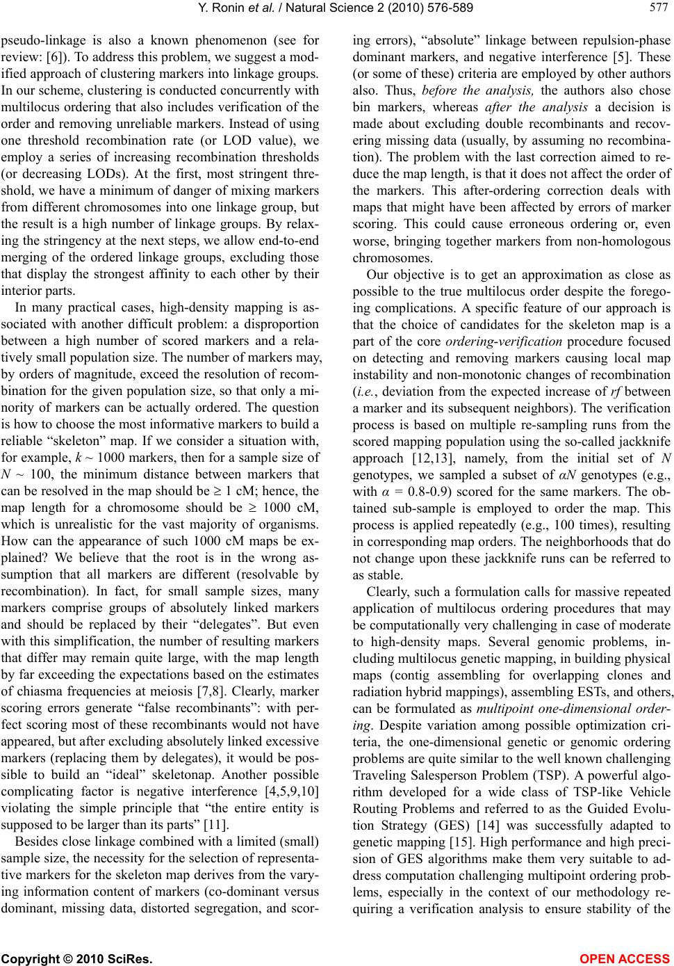

Y. Ronin et al. / Natural Science 2 (2010) 576-589
577
577
pseudo-linkage is also a known phenomenon (see for
review: [6]). To address this problem, we suggest a mod-
ified approach of clustering markers into linkage groups.
In our scheme, clustering is conducted concurrently with
multilocus ordering that also includes verification of the
order and removing unreliable markers. Instead of using
one threshold recombination rate (or LOD value), we
employ a series of increasing recombination thresholds
(or decreasing LODs). At the first, most stringent thre-
shold, we have a minimum of danger of mixing markers
from different chromosomes into one linkage group, but
the result is a high number of linkage groups. By relax-
ing the stringency at the next steps, we allow end-to-end
merging of the ordered linkage groups, excluding those
that display the strongest affinity to each other by their
interior parts.
In many practical cases, high-density mapping is as-
sociated with another difficult problem: a disproportion
between a high number of scored markers and a rela-
tively small population size. The number of markers may,
by orders of magnitude, exceed the resolution of recom-
bination for the given population size, so that only a mi-
nority of markers can be actually ordered. The question
is how to choose the most informative markers to build a
reliable “skeleton” map. If we consider a situation with,
for example, k ~ 1000 markers, then for a sample size of
N ~ 100, the minimum distance between markers that
can be resolved in the map should be  1 cM; hence, the
map length for a chromosome should be  1000 cM,
which is unrealistic for the vast majority of organisms.
How can the appearance of such 1000 cM maps be ex-
plained? We believe that the root is in the wrong as-
sumption that all markers are different (resolvable by
recombination). In fact, for small sample sizes, many
markers comprise groups of absolutely linked markers
and should be replaced by their “delegates”. But even
with this simplification, the number of resulting markers
that differ may remain quite large, with the map length
by far exceeding the expectations based on the estimates
of chiasma frequencies at meiosis [7,8]. Clearly, marker
scoring errors generate “false recombinants”: with per-
fect scoring most of these recombinants would not have
appeared, but after excluding absolutely linked excessive
markers (replacing them by delegates), it would be pos-
sible to build an “ideal” skeletonap. Another possible
complicating factor is negative interference [4,5,9,10]
violating the simple principle that “the entire entity is
supposed to be larger than its parts” [11].
Besides close linkage combined with a limited (small)
sample size, the necessity for the selection of representa-
tive markers for the skeleton map derives from the vary-
ing information content of markers (co-dominant versus
dominant, missing data, distorted segregation, and scor-
ing errors), “absolute” linkage between repulsion-phase
dominant markers, and negative interference [5]. These
(or some of these) criteria are employed by other authors
also. Thus, before the analysis, the authors also chose
bin markers, whereas after the analysis a decision is
made about excluding double recombinants and recov-
ering missing data (usually, by assuming no recombina-
tion). The problem with the last correction aimed to re-
duce the map length, is that it does not affect the order of
the markers. This after-ordering correction deals with
maps that might have been affected by errors of marker
scoring. This could cause erroneous ordering or, even
worse, bringing together markers from non-homologous
chromosomes.
Our objective is to get an approximation as close as
possible to the true multilocus order despite the forego-
ing complications. A specific feature of our approach is
that the choice of candidates for the skeleton map is a
part of the core ordering-verification procedure focused
on detecting and removing markers causing local map
instability and non-monotonic changes of recombination
(i.e., deviation from the expected increase of rf between
a marker and its subsequent neighbors). The verification
process is based on multiple re-sampling runs from the
scored mapping population using the so-called jackknife
approach [12,13], namely, from the initial set of N
genotypes, we sampled a subset of αN genotypes (e.g.,
with α = 0.8-0.9) scored for the same markers. The ob-
tained sub-sample is employed to order the map. This
process is applied repeatedly (e.g., 100 times), resulting
in corresponding map orders. The neighborhoods that do
not change upon these jackknife runs can be referred to
as stable.
Clearly, such a formulation calls for massive repeated
application of multilocus ordering procedures that may
be computationally very challenging in case of moderate
to high-density maps. Several genomic problems, in-
cluding multilocus genetic mapping, in building physical
maps (contig assembling for overlapping clones and
radiation hybrid mappings), assembling ESTs, and others,
can be formulated as multipoint one-dimensional order-
ing. Despite variation among possible optimization cri-
teria, the one-dimensional genetic or genomic ordering
problems are quite similar to the well known challenging
Traveling Salesperson Problem (TSP). A powerful algo-
rithm developed for a wide class of TSP-like Vehicle
Routing Problems and referred to as the Guided Evolu-
tion Strategy (GES) [14] was successfully adapted to
genetic mapping [15]. High performance and high preci-
sion of GES algorithms make them very suitable to ad-
dress computation challenging multipoint ordering prob-
lems, especially in the context of our methodology re-
quiring a verification analysis to ensure stability of the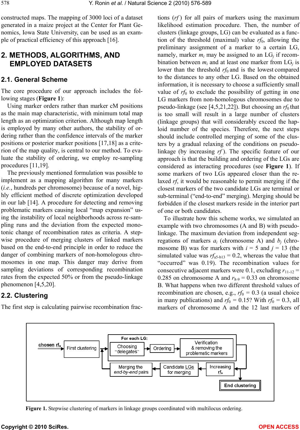

Y. Ronin et al. / Natural Science 2 (2010) 576-589
578
constructed maps. The mapping of 3000 loci of a dataset
generated in a maize project at the Center for Plant Ge-
nomics, Iowa State University, can be used as an exam-
ple of practical efficiency of this approach [16].
2. METHODS, ALGORITHMS, AND
EMPLOYED DATASETS
2.1. General Scheme
The core procedure of our approach includes the fol-
lowing stages (Figure 1):
Using marker orders rather than marker cM positions
as the main map characteristic, with minimum total map
length as an optimization criterion. Although map length
is employed by many other authors, the stability of or-
dering rather than the confidence intervals of the marker
positions or posterior marker positions [17,18] as a crite-
rion of the map quality, is central to our method. To eva-
luate the stability of ordering, we employ re-sampling
procedures [11,19].
The previously mentioned formulation was possible to
implement as a mapping algorithm for many markers
(i.e., hundreds per chromosome) because of a novel, hig-
hly efficient method of discrete optimization developed
in our lab [14]. A procedure for detecting and removing
problematic markers causing local “map expansion” us-
ing the instability of local neighborhoods across re-sam-
pling runs and the deviation from the expected mono-
tonic change of recombination rates as criteria. A step-
wise procedure of merging clusters of linked markers
based on the end-to-end principle in order to reduce the
danger of combining markers of non-homologous chro-
mosomes in one map. This danger may derive from
sampling deviations of corresponding recombination
rates from the expected 50% or from the pseudo-linkage
phenomenon [4,5,20].
2.2. Clustering
The first step is calculating pairwise recombination frac-
tions (rf ) for all pairs of markers using the maximum
likelihood estimation procedure. Then, the number of
clusters (linkage groups, LG) can be evaluated as a func-
tion of the threshold (maximal) value rf0, allowing the
preliminary assignment of a marker to a certain LG,
namely, marker mi may be assigned to an LGj if recom-
bination between mi and at least one marker from LGj is
lower than the threshold rf0 and is the lowest compared
to the distances to any other LG. Based on the obtained
information, it is necessary to choose a sufficiently small
value of rf0 to exclude the possibility of getting in one
LG markers from non-homologous chromosomes due to
pseudo-linkage (see [4,5,21,22]). But choosing an rf0 that
is too small will result in a large number of clusters
(linkage groups) that will considerably exceed the hap-
loid number of the species. Therefore, the next steps
should include controlled merging of some of the clus-
ters by a gradual relaxing of the conditions on pseudo-
linkage (by increasing rf ). The specific feature of our
approach is that the building and ordering of the LGs are
considered as interacting procedures (see Figure 1). If
some markers of two LGs appeared closer than the re-
laxed rf, it would be reasonable to permit merging if the
closest markers of the two candidate LGs are terminal or
sub-terminal (“end-to-end” merging). Merging should be
forbidden if the closest markers reside in the interior part
of one or both candidates.
To illustrate how this scheme works, we simulated an
example with two chromosomes (A and B) with pseudo-
linkage. The maximum deviation from independent seg-
regations of markers ai (chromosome A) and bj (chro-
mosome B) was for markers with i = 5 and j = 13 (the
simulated value was rfa5-b13 = 0.2, whereas the value that
“occurred” was 0.19). The recombination values for
consecutive adjacent markers were 0.1, excluding r11-12 =
0.285 on chromosome A and r8-9 = 0.33 on chromosome
B. What happens when two different threshold values of
recombination are chosen, e.g., rf0 = 0.3 (a usual choice
in many publications) and rf0 = 0.15? With rf0 = 0.3, all
markers of chromosome A and the 12 last markers of
Figure 1. Stepwise clustering of markers in linkage groups coordinated with multilocus ordering.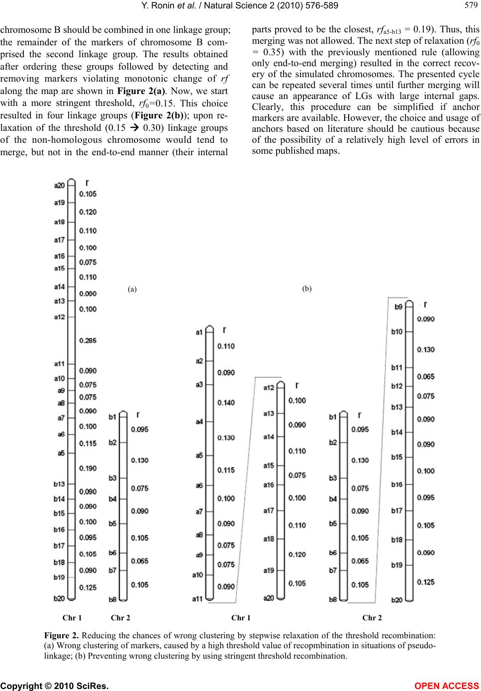

Y. Ronin et al. / Natural Science 2 (2010) 576-589
579
579
chromosome B should be combined in one linkage group;
the remainder of the markers of chromosome B com-
prised the second linkage group. The results obtained
after ordering these groups followed by detecting and
removing markers violating monotonic change of rf
along the map are shown in Figure 2(a). Now, we start
with a more stringent threshold, rf0=0.15. This choice
resulted in four linkage groups (Figure 2(b)); upon re-
laxation of the threshold (0.15  0.30) linkage groups
of the non-homologous chromosome would tend to
merge, but not in the end-to-end manner (their internal
parts proved to be the closest, rfa5-b13 = 0.19). Thus, this
merging was not allowed. The next step of relaxation (rf0
= 0.35) with the previously mentioned rule (allowing
only end-to-end merging) resulted in the correct recov-
ery of the simulated chromosomes. The presented cycle
can be repeated several times until further merging will
cause an appearance of LGs with large internal gaps.
Clearly, this procedure can be simplified if anchor
markers are available. However, the choice and usage of
anchors based on literature should be cautious because
of the possibility of a relatively high level of errors in
some published maps.
(a) (b)
Chr 1 Chr 2 Chr 1Chr 2
Figure 2. Reducing the chances of wrong clustering by stepwise relaxation of the threshold recombination:
(a) Wrong clustering of markers, caused by a high threshold value of recopmbination in situations of pseudo-
linkage; (b) Preventing wrong clustering by using stringent threshold recombination.

Y. Ronin et al. / Natural Science 2 (2010) 576-589
580
2.3. Multilocus Ordering
As noted above, the number of scored markers may, by
orders of magnitude, exceed the number of those practi-
cally resolvable by recombination markers for the given
population size. Only a small portion of markers (here
referred to as delegate markers) can be included in the
skeleton map, with the remaining markers being at-
tached to the delegates. Besides the non-resolvable
linkage caused by small sample size, the necessity for
selection of representative markers for the skeleton map
derives from non-random (clustered) recombination dis-
tribution in the genome [4], varying information content
of the markers (co-dominant versus dominant, missing
data, distorted segregation, and scoring errors), biased
recombination estimates between repulsion-phase
dominant markers [19], and negative interference [5,10].
Using our approach (implemented in MultiPoint package,
http://www.multiqtl.com), one may start from a linkage
group with hundreds of markers and conduct several
analytical steps in order to build a reliable map:
 multilocus ordering;
 binding together closely linked markers followed
by selection of delegates (bin markers) with the
highest information content and replacing the gro-
ups of tightly linked markers by their “delegates”;
repeated ordering and re-sampling verification of
the reduced LG to detect regions of map instabil-
ity;
 removing the markers causing unstable neighbor-
hoods and violating monotonic change of recom-
bination, followed by repeated ordering to obtain
the skeleton map;
 attaching the removed markers to their best inter-
vals on the skeleton map.
Our mapping algorithm is based on the reduction of
the multilocus ordering problem to TSP or TSP-like for-
mulation. Its main features were described earlier [11,
19]. Here we present only recent modifications and ex-
tensions of our ordering algorithm. One of the possibili-
ties in addressing the mapping problem is to recover the
marker order from a known matrix dij of pair-wise
marker distances based on estimates of the recombina-
tion rate. An important fact is that in genetic ordering
problems the distances between the markers cannot be
measured directly. For this reason, even an exact TSP
solution does not guarantee that the obtained map will be
robust to a small variation of the data, hence the impor-
tance of stability testing. Special formulations of the
problem may include various restrictions (e.g., on a pre-
defined order of anchor markers), implying a reduction
of genetic mapping to a more complex constrained dis-
crete optimization problem.
In order to improve the efficiency of our multilocus
ordering algorithms, we developed a new metaheuristic
approach, referred to as the Guided Evolution Strategy
(GES) that combines the strengths of the Guided Local
Search (GLS – [33]) and Evolution Strategies [19] in the
framework of one iterative two-stage procedure. GES
combines the ES and GLS metaheuristics, and these two
stages are iteratively repeated until no more improve-
ments can be found in the local search. Our experiments
on 302 large-scale benchmark vehicle routing problems
with constraints demonstrated that the proposed algo-
rithm is fast, cost-effective, and highly competitive, pro-
ducing the best known solutions to 82% of the con-
strained benchmark problems [14]. We adapted this GES
approach to TSP-like problems of genetic mapping, in-
cluding the Fast2Opt local search procedure and new
variable (adaptive) neighborhood size. The new map-
ping-oriented algorithm works with small neighborhoods
(25-50 neighbor markers) that allows significantly ac-
celerate the performance on large-scale problems. The
algorithm was tested on standard TSPlib problems with
50-2392 points. All known best solutions were achieved
for these problems.
2.4. Map Verification
The objective of the verification procedure is detecting
regions with unstable neighborhoods relative to the initial
ordering (in the following example, explaining the method,
we used 10 markers numbered from 1 to 10). This can be
achieved by repeated re-sampling of the initial dataset
(jackknife, bootstrap) followed by multilocus ordering for
each such derivative sample (Figure 3(a)). Then, the
identification of unstable regions can be conducted based
on the frequency distribution of the right-side and left-side
neighbors (Figures 3(b)-3(d)). The identification of such
regions can be conducted by summing up corresponding
neighborhood matrices (Figures 3(b)-3(c)) and calcu-
lating the neighborhood frequencies (Figure 3(d)). The
higher the deviation from 1 (i.e., from the “diagonal”
pattern) the less certain is local order. In the example, we
show only two re-sampling runs. Based on this small-
size re-sampling, we can indicate certain local neighbor-
hoods, i.e., for marker pairs 1-2, 4-5, 7-8, and 9-10. In
actual analysis the number of runs should be at least a
few dozen or hundreds.
Clearly, the unstable neighborhoods result from fluc-
tuations in the estimates of recombination rates across
the repeated samples; the range of fluctuations depends
on the sample size and the proportion of individuals
taken at each jackknife run. In our framework, jackknife
analysis is a modeling tool to quantify the diversity of
map versions for the treated chromosome representing
the sampling (stochastic) nature of the map. The results
of such an evaluation can facilitate further decision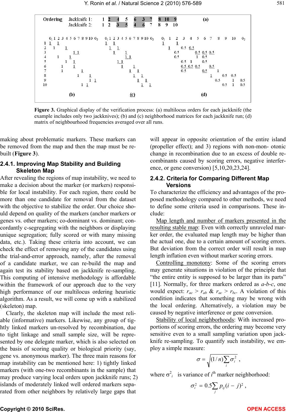

Y. Ronin et al. / Natural Science 2 (2010) 576-589
581
581
Figure 3. Graphical display of the verification process: (a) multilocus orders for each jackknife (the
example includes only two jackknives); (b) and (c) neighborhood matrices for each jackknife run; (d)
matrix of neighbourhood frequencies averaged over all runs.
making about problematic markers. These markers can
be removed from the map and then the map must be re-
built (Figure 3).
2.4.1. Improving Map Stability and Building
Skeleton Map
After revealing the regions of map instability, we need to
make a decision about the marker (or markers) responsi-
ble for local instability. For each region, there could be
more than one candidate for removal from the dataset
with the objective to stabilize the order. Our choice sho-
uld depend on quality of the markers (anchor markers or
genes vs. other markers; co-dominant vs. dominant; con-
cordantly c-segregating with the neighbors or displaying
unique segregation; fully scored or with many missing
data, etc.). Taking these criteria into account, we can
check the effect of removing any of the candidates using
the trial-and-error approach, namely, after the removal
of a candidate marker, we can re-build the map and
again test its stability based on jackknife re-sampling.
This computing of intensive methodology is affordable
within the framework of our approach due to the very
high performance of our multilocus ordering heuristic
algorithm. As a result, we will come up with a stabilized
(skeleton) map.
Clearly, the skeleton map will include the most reli-
able (informative) markers. Likewise, any group of tig-
htly linked markers un-resolved by recombination, due
to tight linkage and small sample size, will be repre-
sented by one delegate marker, which is also selected on
the basis of scoring quality or biological priority (say,
gene vs. anonymous marker). The three main reasons for
map instability can be mentioned here: 1) tightly linked
markers (with one-two recombinants in the sample) that
may produce varying local orders upon jackknife runs; 2)
islands of moderately linked well ordered markers sepa-
rated from other neighbors by relatively large gaps that
will appear in opposite orientation of the entire island
(propeller effect); and 3) regions with non-mon- otonic
change in recombination due to an excess of double re-
combinants caused by scoring errors, negative interfer-
ence, or gene conversion) [5,10,20,23,24].
2.4.2. Criteria for Comparing Different Map
Versions
To characterize the efficiency and advantages of the pro-
posed methodology compared to other methods, we need
to define some criteria used in comparisons. These in-
clude:
Map length and number of markers presented in the
resulting stable map: Even with correctly unraveled mar-
ker order, the evaluated map length may be higher than
the actual one, due to a certain amount of scoring errors.
But deviation from the correct order will result in map
length inflation even without marker scoring errors.
Controlling monotony: Some of the scoring errors
may generate situations in violation of the principle that
“the entire entity is supposed to be larger than its parts”
[11]. Normally, for three markers ordered as a-b-c, one
would expect: rac > r
ab & rac > r bc. A violation of this
condition indicates that something may be wrong with
the local ordering. Alternatively, a violation may be
caused by negative interference or gene conversion.
Stability of local neighborhoods: With increased pro-
portions of scoring errors, the ordering may become very
sensitive even to a small sampling variation upon jack-
knife re-sampling. To quantify such instability, we em-
ploy a simple measure:


i
i
n2 )/1(  ,
where 2
i is variance of ith marker neighborhood:



j
iji jip 22 )(5.0

,

Y. Ronin et al. / Natural Science 2 (2010) 576-589
582
and pij is the proportion of jackknife runs where markers
i and j were adjacent neighbors. The enumeration of
markers is according to the multilocus order obtained on
the entire sample or based on an external order (e.g.,
from the literature). Stable order will give  = 1.
Concordance of segregation distortion within local
neighborhoods: Segregation distortion is a known phen-
omenon caused by various factors [4]. Upon correct or-
dering, one would expect a certain correspondence be-
tween segregation ratios of neighbor markers (segi and
segi+1), namely, a correct order should give smaller val-
ues of the following criterion Si compared to a wrong
order. If the frequency of one of the two classes at a
marker locus in an RIL (dihaploid, or backcross) popula-
tion or one of the homozygotes in F2 is p1, then the
normalized change of segregation ratio from marker i to
i + 1 can be calculated as:
1,
/100  jiii DdsegS
with dsegi = |p2i - p2i+1|, where p2i and p2i+1 are the fre-
quencies of the second marker class for loci i and i + 1
normalized by p1i and p1i+1, and Di,i+1 is the distance (in
cM) between the markers; for F2:
},max{ 133122  iiiii ppppdseg
where p2i and p3i are the normalized frequencies of the
heterozygote and the second homozygote.
2.4.3. Using Real Mapping Data for Illustration
To illustrate the efficiency of the proposed mapping stra-
tegy on real data we selected a few examples of diverse
organisms: wheat, barley, oat, maize, Arabidopsis, mo-
use, rat, and trout using the data available on the web.
The published results for the same datasets were em-
ployed for comparisons with our map versions.
3. RESULTS
An empirical assessment of the proposed analytical fra-
mework, in comparison with other procedures, can be
conducted using both Monte-Carlo simulations and real
data. The validation of the basic properties of our algo-
rithms was provided in our earlier publications using
simulated data [11,19]. Here we demonstrate the advan-
tages of the extended analytical scheme using genome
mapping data on several eukaryotic species: wheat, bar-
ley, oat, maize, Arabidopsis, mouse, rat, and trout. Ob-
viously, our intention is just to illustrate the proposed
approach rather than to revise the published maps. We
believe that a revision of a map, if needed, should be
conducted by the research groups generating the data.
Among the illustrations provided below, the example
on wheat is presented in more detail. The results on the
other examples are summarized in Table 1, using the
case on maize to explain how we compare the published
and de novo constructed maps. One more example, for
the mouse, is summarized in a separate table (Table 2)
due to the fact that besides chromosome 16, our results
for all other chromosomes corresponded well with the
published map. Like with the mouse, our map version
corresponded well with the published version using a
dataset on Arabidopsis. A slight difference was detected
for chromosome 5 only due to the presence of two
markers with high levels of missing data, which caused
problems in the published map and were excluded from
our version (see Table 1).
3.1. Wheat Chromosome 1B
Wheat data from the GrainGenes website (http://wheat.
pw.usda.gov/GG2/quickquery.shtml) on chromosome
1B for the RIL mapping population Synthetic  Opata
with 81 markers were employed (72 markers remained
after deleting absolutely linked markers). The first step
was to check the marker ordering presented on the web.
Using the re-calculated pair-wise rf values transformed
“back” to F1 level, the length of the map (with Kosambi
mapping function) was estimated as L = 444 cM. Based
on re-sampling analysis, the neighborhood stability of
this map was tested and found to be relatively low (Fig-
ure 4(a)-4(c)).
A more stable ordering, at least for a sub-set of mark-
ers (comprising a skeleton map), can be achieved by re-
moving the markers causing the observed instability and
deviation from the (expected) monotonic growth of re-
combination rates along the map around each of the
markers [11]. After such “cleaning”, a skeleton map with
26 markers was obtained (Figure 5(a)). The first and the
last markers proved to be the same, as they were in the
initial map (Figure 5(b)); the map length was reduced
from 444 cM to 138 cM (!), and this was achieved
without deleting “double recombinants” and replacing
missing scores by those that yield non-recombinants.
The improved quality of our map was accomplished by
detecting and removing problematic markers, mainly
with high missing levels. Historically, these markers
were placed onto the map as “second wave” and “third
wave” markers that were characterized much later than
the first groups of markers and for a much smaller sub-
sample of the initial mapping population. Unlike the
total set with 72 markers, the order of our skeleton map
with a subset of 26 markers (see Figure 5(a)) corre-
sponded well with the published map: the relative or-
dering of the markers in Figure 5(b) has only one minor
“inversion” (between markers Xbcd442 (#66) and
Xbcd441 (#64).
3.2. Maize Chromosome 1(IRIL5)
We employed data on IBM302 intercross recombinant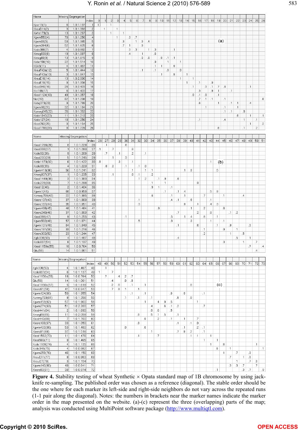

Y. Ronin et al. / Natural Science 2 (2010) 576-589
583
583
Figure 4. Stability testing of wheat Synthetic  Opata standard map of 1B chromosome by using jack-
knife re-sampling. The published order was chosen as a reference (diagonal). The stable order should be
the one where for each marker its left-side and right-side neighbors do not vary across the repeated runs
(1-1 pair along the diagonal). Notes: the numbers in brackets near the marker names indicate the marker
order in the map presented on the website. (a)-(c) represent the three (overlapping) parts of the map;
analysis was conducted using MultiPoint software package (http://www.multiqtl.com).

Y. Ronin et al. / Natural Science 2 (2010) 576-589
584
Figure 5. Stabilizing the map by deriving the skeleton map. The graph represents our trial to stabilize
the wheat 1B map by detecting and removing the markers that caused the local instability of the
neighborhoods. (a) and (b) represent the new (stabilized) and the original (web) versions, respectively.
The order of skeleton markers (which proved to be the “first wave” markers) in our version of the map
displays a remarkable similarity to the order on the website map, excluding one locality.
inbred line (IRIL) mapping population (http://www.
maizegdb.org/cgi-bin/displaymaprecord.cgi?id=870745).
To demonstrate the differences between the web version
and our version of the maps the results on maize chro-
mosome 1 are presented (Table 1). The length of our
version of skeleton map (LMP = 357 cM) is half of that
built with MapMaker (LMM = 696 cM), probably reflect-
ing a better ordering and less discrepancy from the cy-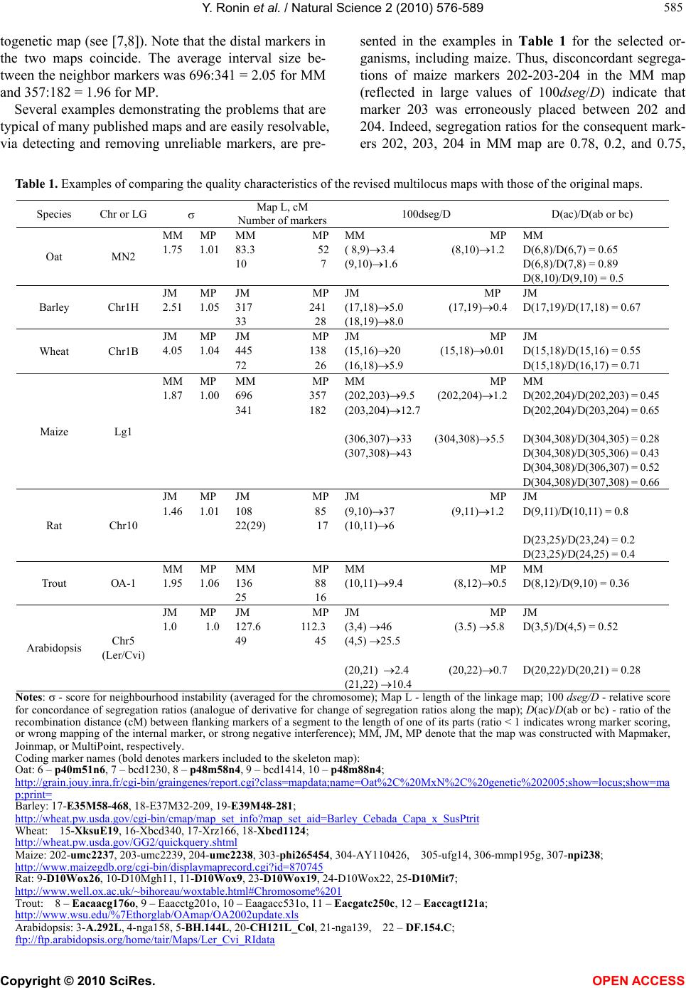

Y. Ronin et al. / Natural Science 2 (2010) 576-589
585
585
togenetic map (see [7,8]). Note that the distal markers in
the two maps coincide. The average interval size be-
tween the neighbor markers was 696:341 = 2.05 for MM
and 357:182 = 1.96 for MP.
Several examples demonstrating the problems that are
typical of many published maps and are easily resolvable,
via detecting and removing unreliable markers, are pre-
sented in the examples in Table 1 for the selected or-
ganisms, including maize. Thus, disconcordant segrega-
tions of maize markers 202-203-204 in the MM map
(reflected in large values of 100dseg/D) indicate that
marker 203 was erroneously placed between 202 and
204. Indeed, segregation ratios for the consequent mark-
ers 202, 203, 204 in MM map are 0.78, 0.2, and 0.75,
Table 1. Examples of comparing the quality characteristics of the revised multilocus maps with those of the original maps.
D(ac)/D(ab or bc) 100dseg/D
Map L, cM
Number of markers
 Chr or LG Species
MM
D(6,8)/D(6,7) = 0.65
D(6,8)/D(7,8) = 0.89
D(8,10)/D(9,10) = 0.5
MM MP
( 8,9)3.4 (8,10)1.2
(9,10)1.6
MM MP
83.3 52
10 7
MM MP
1.75 1.01
MN2 Oat
JM
D(17,19)/D(17,18) = 0.67
JM MP
(17,18)5.0 (17,19)0.4
(18,19)8.0
JM MP
317 241
33 28
JM MP
2.51 1.05 Chr1H Barley
JM
D(15,18)/D(15,16) = 0.55
D(15,18)/D(16,17) = 0.71
JM MP
(15,16)20 (15,18)0.01
(16,18)5.9
JM MP
445 138
72 26
JM MP
4.05 1.04 Chr1B Wheat
MM
D(202,204)/D(202,203) = 0.45
D(202,204)/D(203,204) = 0.65
D(304,308)/D(304,305) = 0.28
D(304,308)/D(305,306) = 0.43
D(304,308)/D(306,307) = 0.52
D(304,308)/D(307,308) = 0.66
MM MP
(202,203)9.5 (202,204)1.2
(203,204)12.7
(306,307)33 (304,308)5.5
(307,308)43
MM MP
696 357
341 182
MM MP
1.87 1.00
Lg1 Maize
JM
D(9,11)/D(10,11) = 0.8
D(23,25)/D(23,24) = 0.2
D(23,25)/D(24,25) = 0.4
JM MP
(9,10)37 (9,11)1.2
(10,11)6
JM MP
108 85
22(29) 17
JM MP
1.46 1.01
Chr10 Rat
MM
D(8,12)/D(9,10) = 0.36
MM MP
(10,11)9.4 (8,12)0.5
MM MP
136 88
25 16
MM MP
1.95 1.06 ОА-1 Trout
JM
D(3,5)/D(4,5) = 0.52
D(20,22)/D(20,21) = 0.28
JM MP
(3,4) 46 (3.5) 5.8
(4,5) 25.5
(20,21) 2.4 (20,22)0.7
(21,22) 10.4
JM MP
127.6 112.3
49 45
JM MP
1.0 1.0
Chr5
(Ler/Cvi)
Arabidopsis
Notes:  - score for neighbourhood instability (averaged for the chromosome); Map L - length of the linkage map; 100 dseg/D - relative score
for concordance of segregation ratios (analogue of derivative for change of segregation ratios along the map); D(ac)/D(ab or bc) - ratio of the
recombination distance (cM) between flanking markers of a segment to the length of one of its parts (ratio < 1 indicates wrong marker scoring,
or wrong mapping of the internal marker, or strong negative interference); ММ, JM, MP denote that the map was constructed with Mapmaker,
Joinmap, or MultiPoint, respectively.
Coding marker names (bold denotes markers included to the skeleton map):
Oat: 6 – p40m51n6, 7 – bcd1230, 8 – p48m58n4, 9 – bcd1414, 10 – p48m88n4;
http://grain.jouy.inra.fr/cgi-bin/graingenes/report.cgi?class=mapdata;name=Oat%2C%20MxN%2C%20genetic%202005;show=locus;show=ma
p;print=
Barley: 17-E35M58-468, 18-E37M32-209, 19-E39M48-281;
http://wheat.pw.usda.gov/cgi-bin/cmap/map_set_info?map_set_aid=Barley_Cebada_Capa_x_SusPtrit
Wheat: 15-XksuE19, 16-Xbcd340, 17-Xrz166, 18-Xbcd1124;
http://wheat.pw.usda.gov/GG2/quickquery.shtml
Maize: 202-umc2237, 203-umc2239, 204-umc2238, 303-phi265454, 304-AY110426, 305-ufg14, 306-mmp195g, 307-npi238;
http://www.maizegdb.org/cgi-bin/displaymaprecord.cgi?id=870745
Rat: 9-D10Wox26, 10-D10Mgh11, 11-D10Wox9, 23-D10Wox19, 24-D10Wox22, 25-D10Mit7;
http://www.well.ox.ac.uk/~bihoreau/woxtable.html#Chromosome%201
Trout: 8 – Eacaacg176o, 9 – Eaacctg201o, 10 – Eaagacc531o, 11 – Eacgatc250c, 12 – Eaccagt121a;
http://www.wsu.edu/%7Ethorglab/OAmap/OA2002update.xls
Arabidopsis: 3-A.292L, 4-nga158, 5-BH.144L, 20-CH121L_Col, 21-nga139, 22 – DF.154.C;
ftp://ftp.arabidopsis.org/home/tair/Maps/Ler_Cvi_RIdata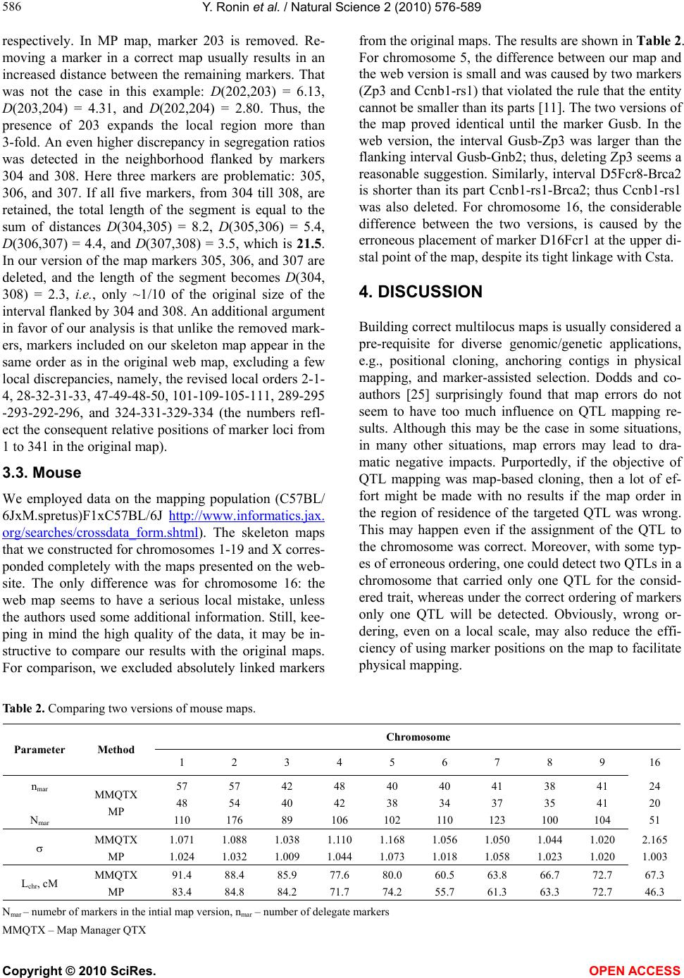

Y. Ronin et al. / Natural Science 2 (2010) 576-589
586
respectively. In МР map, marker 203 is removed. Re-
moving a marker in a correct map usually results in an
increased distance between the remaining markers. That
was not the case in this example: D(202,203) = 6.13,
D(203,204) = 4.31, and D(202,204) = 2.80. Thus, the
presence of 203 expands the local region more than
3-fold. An even higher discrepancy in segregation ratios
was detected in the neighborhood flanked by markers
304 and 308. Here three markers are problematic: 305,
306, and 307. If all five markers, from 304 till 308, are
retained, the total length of the segment is equal to the
sum of distances D(304,305) = 8.2, D(305,306) = 5.4,
D(306,307) = 4.4, and D(307,308) = 3.5, which is 21.5.
In our version of the map markers 305, 306, and 307 are
deleted, and the length of the segment becomes D(304,
308) = 2.3, i.e., only ~1/10 of the original size of the
interval flanked by 304 and 308. An additional argument
in favor of our analysis is that unlike the removed mark-
ers, markers included on our skeleton map appear in the
same order as in the original web map, excluding a few
local discrepancies, namely, the revised local orders 2-1-
4, 28-32-31-33, 47-49-48-50, 101-109-105-111, 289-295
-293-292-296, and 324-331-329-334 (the numbers refl-
ect the consequent relative positions of marker loci from
1 to 341 in the original map).
3.3. Mouse
We employed data on the mapping population (C57BL/
6JxM.spretus)F1xC57BL/6J http://www.informatics.jax.
org/searches/crossdata_form.shtml). The skeleton maps
that we constructed for chromosomes 1-19 and X corres-
ponded completely with the maps presented on the web-
site. The only difference was for chromosome 16: the
web map seems to have a serious local mistake, unless
the authors used some additional information. Still, kee-
ping in mind the high quality of the data, it may be in-
structive to compare our results with the original maps.
For comparison, we excluded absolutely linked markers
from the original maps. The results are shown in Table 2.
For chromosome 5, the difference between our map and
the web version is small and was caused by two markers
(Zp3 and Ccnb1-rs1) that violated the rule that the entity
cannot be smaller than its parts [11]. The two versions of
the map proved identical until the marker Gusb. In the
web version, the interval Gusb-Zp3 was larger than the
flanking interval Gusb-Gnb2; thus, deleting Zp3 seems a
reasonable suggestion. Similarly, interval D5Fcr8-Brca2
is shorter than its part Ccnb1-rs1-Brca2; thus Ccnb1-rs1
was also deleted. For chromosome 16, the considerable
difference between the two versions, is caused by the
erroneous placement of marker D16Fcr1 at the upper di-
stal point of the map, despite its tight linkage with Csta.
4. DISCUSSION
Building correct multilocus maps is usually considered a
pre-requisite for diverse genomic/genetic applications,
e.g., positional cloning, anchoring contigs in physical
mapping, and marker-assisted selection. Dodds and co-
authors [25] surprisingly found that map errors do not
seem to have too much influence on QTL mapping re-
sults. Although this may be the case in some situations,
in many other situations, map errors may lead to dra-
matic negative impacts. Purportedly, if the objective of
QTL mapping was map-based cloning, then a lot of ef-
fort might be made with no results if the map order in
the region of residence of the targeted QTL was wrong.
This may happen even if the assignment of the QTL to
the chromosome was correct. Moreover, with some typ-
es of erroneous ordering, one could detect two QTLs in a
chromosome that carried only one QTL for the consid-
ered trait, whereas under the correct ordering of markers
only one QTL will be detected. Obviously, wrong or-
dering, even on a local scale, may also reduce the effi-
ciency of using marker positions on the map to facilitate
physical mapping.
Table 2. Comparing two versions of mouse maps.
Chromosome
16 9 8 7 6 5 4 3 2 1
Method Parameter
24
20
51
41
41
104
38
35
100
41
37
123
40
34
110
40
38
102
48
42
106
42
40
89
57
54
176
57
48
110
MMQTX
MP
nmar
Nmar
2.165
1.003
1.020
1.020
1.044
1.023
1.050
1.058
1.056
1.018
1.168
1.073
1.110
1.044
1.038
1.009
1.088
1.032
1.071
1.024
MMQTX
MP

67.3
46.3
72.7
72.7
66.7
63.3
63.8
61.3
60.5
55.7
80.0
74.2
77.6
71.7
85.9
84.2
88.4
84.8
91.4
83.4
MMQTX
MP
Lchr, cM
Nmar – numebr of markers in the intial map version, nmar – number of delegate markers
MMQTX – Map Manager QTX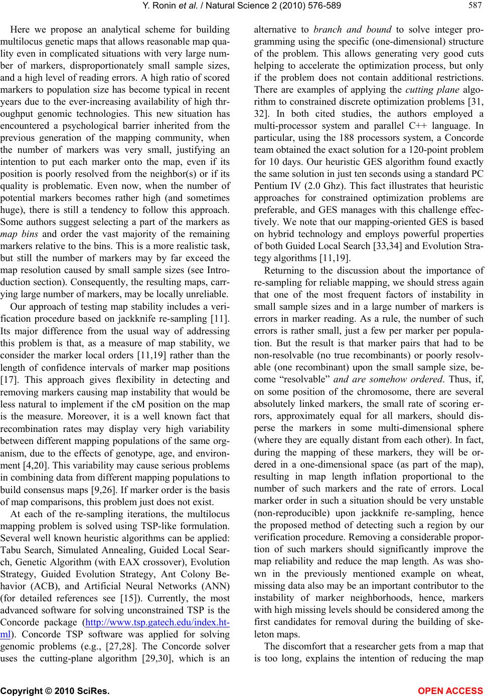

Y. Ronin et al. / Natural Science 2 (2010) 576-589
587
587
Here we propose an analytical scheme for building
multilocus genetic maps that allows reasonable map qua-
lity even in complicated situations with very large num-
ber of markers, disproportionately small sample sizes,
and a high level of reading errors. A high ratio of scored
markers to population size has become typical in recent
years due to the ever-increasing availability of high thr-
oughput genomic technologies. This new situation has
encountered a psychological barrier inherited from the
previous generation of the mapping community, when
the number of markers was very small, justifying an
intention to put each marker onto the map, even if its
position is poorly resolved from the neighbor(s) or if its
quality is problematic. Even now, when the number of
potential markers becomes rather high (and sometimes
huge), there is still a tendency to follow this approach.
Some authors suggest selecting a part of the markers as
map bins and order the vast majority of the remaining
markers relative to the bins. This is a more realistic task,
but still the number of markers may by far exceed the
map resolution caused by small sample sizes (see Intro-
duction section). Consequently, the resulting maps, carr-
ying large number of markers, may be locally unreliable.
Our approach of testing map stability includes a veri-
fication procedure based on jackknife re-sampling [11].
Its major difference from the usual way of addressing
this problem is that, as a measure of map stability, we
consider the marker local orders [11,19] rather than the
length of confidence intervals of marker map positions
[17]. This approach gives flexibility in detecting and
removing markers causing map instability that would be
less natural to implement if the cM position on the map
is the measure. Moreover, it is a well known fact that
recombination rates may display very high variability
between different mapping populations of the same org-
anism, due to the effects of genotype, age, and environ-
ment [4,20]. This variability may cause serious problems
in combining data from different mapping populations to
build consensus maps [9,26]. If marker order is the basis
of map comparisons, this problem just does not exist.
At each of the re-sampling iterations, the multilocus
mapping problem is solved using TSP-like formulation.
Several well known heuristic algorithms can be applied:
Tabu Search, Simulated Annealing, Guided Local Sear-
ch, Genetic Algorithm (with EAX crossover), Evolution
Strategy, Guided Evolution Strategy, Ant Colony Be-
havior (ACB), and Artificial Neural Networks (ANN)
(for detailed references see [15]). Currently, the most
advanced software for solving unconstrained TSP is the
Concorde package (http://www.tsp.gatech.edu/index.ht-
ml). Concorde TSP software was applied for solving
genomic problems (e.g., [27,28]. The Concorde solver
uses the cutting-plane algorithm [29,30], which is an
alternative to branch and bound to solve integer pro-
gramming using the specific (one-dimensional) structure
of the problem. This allows generating very good cuts
helping to accelerate the optimization process, but only
if the problem does not contain additional restrictions.
There are examples of applying the cutting plane algo-
rithm to constrained discrete optimization problems [31,
32]. In both cited studies, the authors employed a
multi-processor system and parallel C++ language. In
particular, using the 188 processors system, a Concorde
team obtained the exact solution for a 120-point problem
for 10 days. Our heuristic GES algorithm found exactly
the same solution in just ten seconds using a standard PC
Pentium IV (2.0 Ghz). This fact illustrates that heuristic
approaches for constrained optimization problems are
preferable, and GES manages with this challenge effec-
tively. We note that our mapping-oriented GES is based
on hybrid technology and employs powerful properties
of both Guided Local Search [33,34] and Evolution Stra-
tegy algorithms [11,19].
Returning to the discussion about the importance of
re-sampling for reliable mapping, we should stress again
that one of the most frequent factors of instability in
small sample sizes and in a large number of markers is
errors in marker reading. As a rule, the number of such
errors is rather small, just a few per marker per popula-
tion. But the result is that marker pairs that had to be
non-resolvable (no true recombinants) or poorly resolv-
able (one recombinant) upon the small sample size, be-
come “resolvable” and are somehow ordered. Thus, if,
on some position of the chromosome, there are several
absolutely linked markers, the small rate of scoring er-
rors, approximately equal for all markers, should dis-
perse the markers in some multi-dimensional sphere
(where they are equally distant from each other). In fact,
during the mapping of these markers, they will be or-
dered in a one-dimensional space (as part of the map),
resulting in map length inflation proportional to the
number of such markers and the rate of errors. Local
marker order in such a situation should be very unstable
(non-reproducible) upon jackknife re-sampling, hence
the proposed method of detecting such a region by our
verification procedure. Removing a considerable propor-
tion of such markers should significantly improve the
map reliability and reduce the map length. As was sho-
wn in the previously mentioned example on wheat,
missing data also may be an important contributor to the
instability of marker neighborhoods, hence, markers
with high missing levels should be considered among the
first candidates for removal during the building of ske-
leton maps.
The discomfort that a researcher gets from a map that
is too long, explains the intention of reducing the map

Y. Ronin et al. / Natural Science 2 (2010) 576-589
588
length, sometimes by rather artificial approaches. For
example, such trials may include removing double re-
combinants and/or recovering the missing data by scores
yielding non-recombinant genotypes after the marker
ordering was finished. We found a good example for
such a situation in re-analyzing the data on wheat chro-
mosome 1B (see the previously mentioned analysis on
wheat chromosome 1B). In a trial to display the map len-
gth for the multilocus order of 1B presented on the web-
site, we used “per meiosis” recombination rates con-
verted to Kosambi map distances. This resulted in a 1B
map with L = 432 cM length, in contrast to the one pub-
lished on the website with L = 104 cM. How could this
huge discrepancy (432 vs. 104 cM) be explained? We
managed to “reproduce” the underlying procedure with
very high precision. As with many other published maps,
major efforts have been invested by several teams to enr-
ich this population with molecular markers from other
populations, thereby bridging these mapping resources
together. Unfortunately, new waves of markers were
scored only partially, so that the level of missing data for
this population was often very high, up to 50-70%.
It appeared that the problem of missing data was
treated by the map constructors (or by the software they
have employed) as follows. After ordering the markers,
missing data were recovered by replacing the missing
scores with those that resulted exclusively in non-re-
combinants. Clearly, the higher the level of missing data
the stronger the effect of such correction will be, i.e., a
reduction of the map length. Before transforming rf val-
ues for RIL to rf values for F1, double recombinants for
any pair of adjacent intervals were also replaced by
non-recombinants. This method of removing erroneous
double recombinants seems reasonable for F2 or double
haploids, but it is inappropriate given that in RIL map-
ping population, “double recombinants” are not neces-
sarily a result of scoring errors or real double recombi-
nation events. Indeed, a considerable portion of “double
recombinants” have likely resulted from recombination
in adjacent intervals that occurred in meiosis IN DIF-
FERENT generations of genotypes that remained het-
erozygous for those regions (in F2, F3, etc.). We consid-
ered several intervals, where our ordering was exactly
the same as in the published map, but the distances were
different (namely, our distances were higher than those
published on the website). After conducting the previ-
ously mentioned “correction” steps, we obtained exac-
tly the same distances as reported on the website map.
The conducted revision analysis indicates that these dis-
tances may be irrelevant to the actual situation. Thus, the
relatively small lengths of those maps are almost cer-
tainly an artifact introduced during the merging of dif-
ferent marker data sources, some of which contained
high frequencies of missing data and inappropriate “er-
ror correction”.
In genetic mapping, multilocus ordering is usually co-
nsidered as a much more complicated problem compared
to subdivision of the marker set into linkage groups.
However, many examples indicate that markers from
non-homologous chromosomes were assigned to the
wrong chromosomes, presumably, due to pseudo-linkage.
We have encountered these types of errors in analyzing
cereal species (see [5]). Similarly, in cattle, such wrong
assignments were found for 12% of markers/contigs (H.
Lewin, personal communication). Thus, the pseudo-lin-
kage phenomenon should be of special concern for
large-scale genetic mapping. As indicated above, incor-
rect assignments can be caused by biological and statis-
tical reasons. The probability of sampling deviation from
the random segregation of markers from non-homolog-
ous chromosomes should grow with increased numbers
of chromosomes, length of chromosomes, number of
markers, and with small sample size. We propose in this
paper that a considerable part of “wrong assignment”
errors can be reduced by the algorithm of stepwise clus-
tering markers into linkage groups alternated by multi-
locus ordering.
The possibility of re-sampling based on testing map
stability by detecting and removing the markers that
cause low map quality is the second major component of
the proposed approach. Detection and removal of the
markers responsible for local map instabilities and
non-monotonic change in recombination rates allows
building stable skeleton maps with minimal total length.
Clearly, there is some degree of uncertainty in such
choices; hence, there might be different versions of the
skeleton map. In such situations, the high performance
of our algorithms is an important advantage allowing
further fast correction (complementing) of the skeleton
map by using additional markers and/or some of the de-
leted markers. Further improvement of the mapping
quality is achievable by joint analysis of mapping data
from different mapping populations that can be referred
to as consensus mapping [9,26].
5. ACKNOWLEDGEMENTS
The study was supported by the Israeli Ministry of Absorption and the
United States-Israel Binational Agricultural Research and Develop-
ment Foundation (grant # 3873-06).
REFERENCES
[1] Lander, E.S. and Green, P. (1987) Construction of multi-
locus linkage maps in human. Proceedings of the Na-
tional Academy of Science, USA, 84(8), 2363-2367.
[2] Stam, P. (1993) Construction of integrated genetic link-

Y. Ronin et al. / Natural Science 2 (2010) 576-589
589
589
age maps by means of a new computer package: JoinMap.
Plant Journal, 3(5), 739-744.
[3] Sapre, A.B. and Deshpande, D.S. (1987) Spontaneous
emergence of parents from the F1 interspecific hybrids of
Coix L. Journal of Heredity, 78(6), 357-360
[4] Korol, A.B., Preygel, I.A. and Preygel, S.I. (1994) Re-
combination variability and evolution. Chapman & Hall,
London.
[5] Peng, J., Korol, A.B., Fahima, T., Roder M.S., Ronin, Y.
I., Li, Y.C. and Nevo, E. (2000) Molecular genetic maps
in wild emmer wheat, Triticum dicoccoides: Genome-
wide coverage, massive negative interference, and puta-
tive quasi-linkage. Genome Research. 10(10), 1509-1531.
[6] Korol, A.B., Shirak, A., Cnaani, A. and Hallerman, E.M.
(2007) Detection and analysis of QTLs for economic
traits in aquatic species. In: Liu, Z.J., Ed., Aquaculture
Genome Technologies. Blackwell, Oxford, 169-197.
[7] Nilsson, N.O., Säll, T. and Bengtsson, B.O. (1993) Chi-
asma and recombination data in plants: Are they com-
patible? Trends in Genetics, 9(10), 344-348.
[8] Anderson, L.K., Doyle, G.G., Brigham, B., Carter, J.,
Hooker, K.D., Lai, A., Rice, M. and Stack, S.M. (2003)
High-resolution crossover maps for each bivalent of Zea
mays using recombination nodules. Genetics, 165(2),
849-865.
[9] Korol, A.B., Mester, D., Frenkel, Z. and Ronin, Y.I.
(2009) Methods for genetic analysis in the Triticeae.
Chapter 6, In: Feuillet, C. and Muehlbauer, G.J., Eds.,
Genetics and Genomics of the Triticeae. Springer, Berlin,
pp. 163-199.
[10] Esch, E., and Weber, W.E. (2002) Investigation of cross-
over interference in barley (Hordeum vulgare L.) using
the coefficient of coincidence. Theoretical and Applied
Genetics, 104(5), 786-796.
[11] Mester, D., Ronin, Y., Minkov, D., Nevo, E. and Korol, A.
(2003b) Constructing large scale genetic maps using an
evolutionary strategy algorithm. Genetics, 165(4), 2269-
2282.
[12] Efron, B. (1979) Bootstrap method: Another look at the
jackknife. The Annals of Statistics, 7(1), 1-26.
[13] Efron, B. and Tibshirani, R.J. (1993) An introduction to
the bootstrap. Chapman and Hall, New York.
[14] Mester, D. and Braysy, O. (2005) Active guided evolu-
tion strategies for large-scale vehicle routing problems
with time windows. Computers & Operation Research
32(6), 1593-1614.
[15] Mester, D.I., Ronin, Y.I., Nevo, E. and Korol, A.B. (2004)
Fast and high precision algorithms for optimization in
large scale genomic problems. Computational Biology
and Chemistry, 28(4), 281-290.
[16] Fu, Y., Wen, T.J., Ronin, Y.I., Chen, H.D., Guo, L.,
Mester, D.I., Yang, Y.J., Lee, M., Korol, A.B., Ashlock D.
A., et al. (2006) Genetic dissection of maize intermated
recombinant inbred lines. Genetics, 174(3), 1671-1683.
[17] Liu, B.H. (1998) Statistical genomics: Linkage, mapping,
and QTL analysis. CRC Press, New York.
[18] Jansen, J., de Jong, A.G. and Ooijen, J.W. (2001) Constr-
ucting dense genetic linkage maps. Theoretical and Ap-
plied Genetics, 102(6-7), 1113-1122.
[19] Mester, D.I., Ronin, Y.I., Hu, Y., Peng, J., Nevo, E. and
Korol, A.B. (2003a) Efficient multipoint mapping: Mak-
ing use of dominant repulsion-phase markers. Theoretical
and Applied Genetics, 107(6), 1002-1112.
[20] Korol, A.B. (2001) Recombination. In: Encyclopedia of
Biodiversity. Academic Press, San Diego, 5, 53-71.
[21] Sakamoto, T., Danzmann, R.G., Gharbi, K., Howard, P.,
Ozaki, A., Khoo, S.K., Woram, R.A., Okamoto, N., Fer-
guson, M.M., Holm, L.E., et al. (2000) A microsatellite
linkage map of rainbow trout (Oncorhynchus mykiss)
characterized by large sex-specific differences in recom-
bination rates. Genetics, 155(3), 1331-1345.
[22] Sivagnanasundaram, S., Broman, K.W., Liu, M. and
Petronis, A. (2004) Quasi-linkage: A confounding factor
in linkage analysis of complex diseases? Hum Genet,
114(6), 588-593.
[23] Morrell, P.L., Toleno, D.M., Lundy, K.E., and Clegg, M.
T. (2006) Estimating the contribution of mutation, re-
combination and gene conversion in the generation of
haplotypic diversity. Genetics, 173(3), 1705-1723.
[24] Plagnol, V., Padhukasahasram, B., Wall, J.D., Marjoram,
P. and Nordborg, M. (2006) Relative influences of cross-
ing over and gene conversion on the pattern of linkage
disequilibrium in Arabidopsis thaliana. Genetics, 172(4),
2441-2448.
[25] Dodds, K.G., Ball, R., Djorovic, N. and Carson, S.D.
(2004) The effect of an imprecise map on interval map-
ping QTLs. Genetical Research, 84(1), 47-55.
[26] Mester, D.I., Ronin, Y.I., Korostishevsky, M.A., Pikus, V.
L., Glazman, A.E. and Korol, A.B. (2006) Multilocus
consensus genetic maps (MCGM): Formulation, algo-
rithms, and results. Computational Biology and Chemis-
try, 30(1), 12-20.
[27] Hitte, C., Lorentzen, T.D., Guyon, R., Kim, L., Cadieu,
E., Parker, H.G., Quignon, P., Lowe, J.K., Gelfenbeyn, B.,
Andre, C., et al. (2003) Comparison of multimap and
TSP/CONCORDE for constructing radiation hybrid
maps. Journal of Heredity, 94(1), 9-13.
[28] Menotti-Raymond, M., David, V.A., Chen, Z.Q., Menotti,
K.A., Sun, S., Schaffer, A.A., Agarwala, R., Tomlin, J.F.,
O’Brien, S.J. and Murphy, W.J. (2003) Second-genera-
tion integrated genetic linkage/radiation hybrid maps of
the domestic cat (Felis catus). Journal of Heredity, 94(1),
95-106.
[29] Dantzig, G., Fulkerson, R. and Johnson, S. (1954) Solu-
tion of a large-scale traveling salesman problem. Opera-
tions Research, 2, 393-410.
[30] Appligate, D., Bixby, R., Chvatal V. and Cook, W. (1998)
On the solution of traveling salesman problem. Docu-
menta Mathematica, Extra Volume International Con-
gress of Mathematics III, 645-656.
[31] Cook, W. and Rich, J.L. (1999) A parallel cutting-plane
algorithm for vehicle routing problem with time window.
Grant Working, Princeton University, USA.
[32] Appligate, D., Cook, W., Dash, S. and Rohe, A. (2002)
Solution of min-max vehicle routing problem. INFO-
RMS Journal on Computing, 14(2), 132-143.
[33] Voudouris, C. (1997) Guided local search for combinato-
rial problems. Ph.D. thesis, Department of Computer Sci-
ence, University of Essex, Colchester.
[34] Tsang, E. and Voudouris, C. (1997) Fast local search and
guided local search and their application to British tele-
com’s workforce scheduling problem. Operations Re-
search Letters, 20(3) , 119-127.