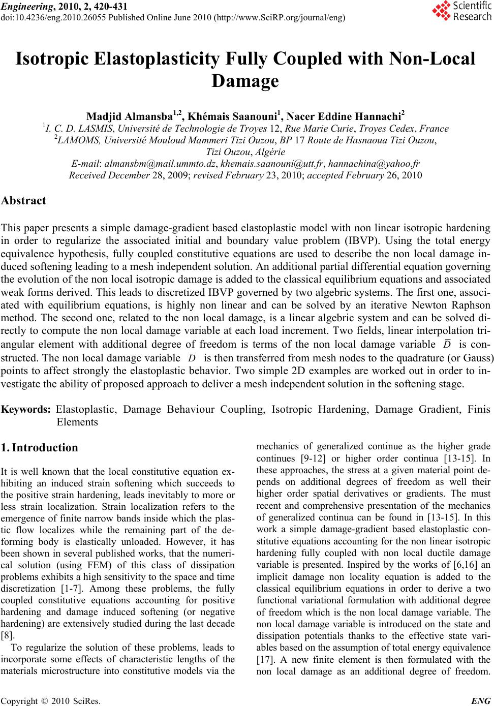Engineering, 2010, 2, 420-431
doi:10.4236/eng.2010.26055 Published Online June 2010 (http://www.SciRP.org/journal/eng)
Isotropic Elastoplasticity Fully Coupled with Non-Local
Damage
Madjid Almansba1,2, Khémais Saanouni1, Nacer Eddine Hannachi2
1I. C. D. LASMIS, Université de Technologie de Troyes 12, Rue Marie Curie, Troyes Cedex, France
2LAMOMS, Université Mouloud Mammeri Tizi Ouzou, BP 17 Route de Hasnaoua Tizi Ouzou,
Tizi Ouzou, Algérie
Received December 28, 2009; revised February 23, 2010; accepted February 26, 2010
Abstract
This paper presents a simple damage-gradient based elastoplastic model with non linear isotropic hardening
in order to regularize the associated initial and boundary value problem (IBVP). Using the total energy
equivalence hypothesis, fully coupled constitutive equations are used to describe the non local damage in-
duced softening leading to a mesh independent solution. An additional partial differential equation governing
the evolution of the non local isotropic damage is added to the classical equilibrium equations and associated
weak forms derived. This leads to discretized IBVP governed by two algebric systems. The first one, associ-
ated with equilibrium equations, is highly non linear and can be solved by an iterative Newton Raphson
method. The second one, related to the non local damage, is a linear algebric system and can be solved di-
rectly to compute the non local damage variable at each load increment. Two fields, linear interpolation tri-
angular element with additional degree of freedom is terms of the non local damage variable D is con-
structed. The non local damage variable D is then transferred from mesh nodes to the quadrature (or Gauss)
points to affect strongly the elastoplastic behavior. Two simple 2D examples are worked out in order to in-
vestigate the ability of proposed approach to deliver a mesh independent solution in the softening stage.
Keywords: Elastoplastic, Damage Behaviour Coupling, Isotropic Hardening, Damage Gradient, Finis
Elements
1. Introduction
It is well known that the local constitutive equation ex-
hibiting an induced strain softening which succeeds to
the positive strain hardening, leads inevitably to more or
less strain localization. Strain localization refers to the
emergence of finite narrow bands inside which the plas-
tic flow localizes while the remaining part of the de-
forming body is elastically unloaded. However, it has
been shown in several published works, that the numeri-
cal solution (using FEM) of this class of dissipation
problems exhibits a high sensitivity to the space and time
discretization [1-7]. Among these problems, the fully
coupled constitutive equations accounting for positive
hardening and damage induced softening (or negative
hardening) are extensively studied during the last decade
[8].
To regularize the solution of these problems, leads to
incorporate some effects of characteristic lengths of the
materials microstructure into constitutive models via the
mechanics of generalized continue as the higher grade
continues [9-12] or higher order continua [13-15]. In
these approaches, the stress at a given material point de-
pends on additional degrees of freedom as well their
higher order spatial derivatives or gradients. The must
recent and comprehensive presentation of the mechanics
of generalized continua can be found in [13-15]. In this
work a simple damage-gradient based elastoplastic con-
stitutive equations accounting for the non linear isotropic
hardening fully coupled with non local ductile damage
variable is presented. Inspired by the works of [6,16] an
implicit damage non locality equation is added to the
classical equilibrium equations in order to derive a two
functional variational formulation with additional degree
of freedom which is the non local damage variable. The
non local damage variable is introduced on the state and
dissipation potentials thanks to the effective state vari-
ables based on the assumption of total energy equivalence
[17]. A new finite element is then formulated with the
non local damage as an additional degree of freedom.

M. ALMANSBA ET AL.421
This leads to two algebric systems, one highly non linear
and the other is quite linear giving a non local damage at
each load increment. Some simple examples are per-
formed in order to show the ability of the proposed ap-
proach to avoid the mesh dependency of the solution of
the IBVP.
2. On Isotropic Elasto-Plasticity with
Damage-Gradient
In previous works [8,18] the authors have proposed ad-
vanced constitutive equations for sheet or balk metal
forming accounting for thermal effect, elasto (visco) pla-
sticity, mixed non linear hardening, isotropic ductile
damage and contact with friction. These fully coupled
multiphysics models has been formulating, in the frame-
work of the thermodynamics of irreversible processes
assuming a fully local theory in which only the first gra-
dient of the displacement is required. In this work, a non
local damage variable ()D is introduced in these con-
stitutive equations replacing the classical local damage
variable (D) by the non local damage variable ()D
solution of the following partial differential equation [6]:


0 in (a)
grad.0 in (b)
D
D
DdivD
Dn

 





  (1)
The Equation (1(b)) represents the Neumann type
boundary condition prescribed on the boundary
D

of
the damaged volume
D
 and ω is homogeneous to a
length squared and plays the role of an internal character-
istic length of material, governing the non-locality of the
damage field. This leads to introduce the damage gradient
in the classical local constitutive equations in order to
regularize the initial boundary value problem (IBVP) with
respect to the space and time discretization. For the sake
of simplicity we limit resolves to the fully isotropic and
isothermal elastoplasticity assuming the von Mises yield
function and non linear isotropic hardening assuming the
small strain hypothesis.
2.1. Constitutive Model for Plasticity with
Isotropic Hardening and Non Local
Damage
Following the idea by [19], the non local damage vari-
able is computed from Equation (1) and introduced into
the local constitutive equations simply by replacing the
local damage variable (D) by ()D. The complete set of
these constitutive equations fully coupled with non local
damage variable is then given by:


 
1 :
1 :
e
p
D
D



 
  1
pn
D




 (2)


1 RDQr (1r1)
1
rb
D




D (3)
2
11
::
22
ee
YQr  

0
1
s
YY
DS
D

 


 (4)
where “

” is the Cauchy’s stress tensor,

is the
stiffness tensor, “e

” the elastic strain tensor, “
p

” is
the plastic strain, R and r are respectively the isotropic
stress and its isotropic strain, “Q” is the isotropic hard-
ening modulus and “b” is non-linearity parameter of
the isotropic hardening. “Y” the thermodynamic force
associated to the local damage “D” which resolves ac-
cording to Equation (4(b)), in which S, s,

and Y0 are
the ductile damage parameters. The deviatoric tensors n
and n
 define the outward unit normal to the yield func-
tion f = 0 in the stress and effective stress spaces respec-
tively. They are defined by:
31 1
2111
f
Sf
n
DD


 

n
D



 (5)
In these equations “

” is the classical plastic multi-
plier derived from the consistency condition applied to
the yield function:
1y
R
f
D





 (6)
in which “y

” is the flow stress in simple tension
and 3:
2SS
  is the von Mises equivalent stress:

1.1
3
Str 






. If the analytic form of


if
is de-
duced from the consistency condition ,

0 0ff

one can obtain


DD
:
31 : 1 0 0
0 else where
e
pD
DS iffand f
HS












(7)
where

ˆ
31 12
1
y
pD e
R
HDQbRDY
D







is the elastoplastic hardening modulus. With ˆ Y



0
1
1
s
YY
S
D



. From numerical point of view, Equ-
ation (7) is not needed since is taken as the
t   


M. ALMANSBA ET AL. 422
principal unknown to be computed from 0
tt
f
 
t
at the
end of each time increment .
1nn
tt

 
3. Numerical Aspects
As discussed above the initial and boundary value prob-
lem is driven by the partial differential equations (PDEs)
describing both the equilibrium problem (the inertia be-
ing neglected) and the damage non locality equation
(Equation (1
)):

F
u
in (a
in (b
in (c
0
.
v
div f
nF
Uu


)
)
)















(8)
where v
f
 is the body forces vector. is the outward
normal to the boundary
n

F
 where the forces vectors
F

is prescribed ; while is the boundary of the
u


where the displacement u

vector is prescribed

uF
 
¨the boundary of  and

uF
 .
Both Equation (1) and Equation (8) will be solved us-
ing the “displacement” based Galerkin finite element
method is discussed here after.
3.1. Variation Formulation and Global
Resolution Scheme
Let u

 the virtual displacement vector and D

the
virtual non local damage both compatible with the boun-
dary conditions (i.e. kinematically admissible (K.A)).
The weak forms associated with Equation (1) and Equa-
tion (8) are easily deduced:





, u:
..0 A
, D.
0
F
D
u K.
D K.A
D
u
v
D
Iu ud
uf duFds
IDD DD
DDd

 





Dd 


 

 

















 

 


(9)
Since the domain  is discretized into many sub-do-
mains (or finites elements) e, then the elementary weak
forms written on each element (e) lead to:




, u:
, D
e
Fe
e
D
e
D
ee ee
ue
ee
ev e
ee eee
D
e
e
Iu ud
uFdsf ud
I
DDDD
DDd








Consequently, the system (9) can be written under the
following discretized when the do main  is discretized
into “Nele” elements from:
1
1
u K.A.
D K.A.
Nele
e
uu
e
Nele
e
DD
e
II
II














(11)
By using the Bubnov-Galerkin method, the real and
virtual quantities are approximated over each finite ele-
ment (e) according to (the matrix notations will he used):






  
eee eee
unu n
eee ee
nn
DD
uNu uNu
DND DND


 

 
 

 
e
(12)
where e
u
N



 and e
D
N



 are the matrices of the shape
functions relative to the nodal unknown


e
u and


e
D. Their first gradients are then deduced:
  
 
u
u
D
D
e
eeee
nn
j
e
e
ee
nn
j
NuBu
x
N
DDBD
xx



  






 
 



 


e
(a)
  
 
u
u
D
D
e
eee
nn
j
e
e
ee
nn
j
NuBu
x
N
DDBD
xx
 



  


 


 
 







e
e
(b)
(13)
Introducing Equation (12) and Equation (13) in Equa-
tion (10) leads to:
Dd

 



















 

  (10)









.
..
e
ee
e
e
e
ue
ee e
un
TT
ee
ueue
T
eee
k
DDD
ee e
n DT
e
e
D
Bd
Iuu
NTds Nfd
BBNDd
IDD
NDd
















 

 






 


 























(14)
In Equation (14(b)) [] is the diagonal matrix of in-
ternal lengths.

2
2
2
0..0
:..
:..::
00..
l
l
l

0















(15)

M. ALMANSBA ET AL. 423





DD
D
TT
eeee
jDDD
Npg
T
ee
jD
Npg
KBBN
FNDJ



After the standard assembly operation, the following e
D
N












(18)
algebric system written at is obtained:
1n
t
  

 


1int
1
1
1
=0 (a)
=0 (b)
D
DD
ee
next
en
ee
n
en
RFF
HKDF


















(16)
where the integrals entering the matrix e
DD
K

 
and the
vectors , and

int
e
F

t
e
ex
F

e
D
F
can be written
with the help of Newton integration method, as follows:




 
int
T
ee
ju
Npg
T
ee e
T
j
uju
ext Npg Npg
FBJ
s
F
NfJ NTJ




 

 


(17)
From Equation (16) it is worth noting that if the
first Equation (16(a)) is highly non linear and should be
solved iteratively, the second one Equation (16(b)) is
perfectly linear an can be solved directly without any
iterative procedure [20]. For this end, a 2D plane strain
simple linear (triangle) element is constructed with three
degrees of freedom (dof) per node namely two displace-
ment components (u, v) and the non local damage (D).
Since the dof’s (u, v) are independent from dof (D),
similar linear approximation is assumed for both (u,v)
and (D). Accordingly a very classical triangular isopa-
rametric element with a single integration point is used.
The Figure 1 summarizes the resolution scheme used
No Yes
Increment : t=t+

t
Compute
 
1
111
hh
nnn
u



 
Compute {} from

1h
u


Compute






11 1
, ,
nn n
RD 
 
Compute
 
11
int 11
,
hh
ext
nn
FF




Compute
 
111
int
111
hhh
ext
nnn
RF F





Convergence test
Else
  
1 11
11
h hh
T
nn
uKR
 


Solver for


1n
D





1
1DD n n
DKD




Itération : h+1
Time t=t+1
Figure 1. Flow chart of the global resolution scheme.

M. ALMANSBA ET AL. 424
in this work to solve Equation (16).
3.2. Local Integration Scheme
At each time, the calculation of the internal forces
in Equation (17(a)) and
1n
t

int
e
F

D
e
F
in Equation
(18(b)) needs the computation of the stress

1n


and
local damage

. This is done through the numerical
integration of the fully coupled constitutive equations
presented above Equation (2) to Equation (4). The stan-
dard elastic prediction and plastic correction algorithm
[8,21,22] is used for computation of the stress tensor
together with the other state variables of the model.
1n
D
3.2.1. Elastic Prediction
Elastic prediction stage consists to assume that the given
total strain increment is elastic without any dissipation
(i.e. 0.

 ). This leads to define the “trial” stress as:

**
1
1:
nn
D1
n



 (19)
where *
11
p
nn n



  is the known trial strain su-
pposed as purely elastic. The “trial” yield function is
then defined by:
*
1
*
11
nn
n
n
R
f
D

y






(20)
The non local damage “D” at each integration point
is obtained by linear interpolation from the nodes and is
kept contort equal to “n D” during the iterative resolution
of the equilibrium equations:
If the solution is effectively elastic and the
solution is:
*
1<0 n
f
*
111 11
, , ,
pp
nnnnnnn
RR DD  
 
 n  (21)
If , the trial solution should corrected in order
to fulfill the yield criterion.
*
1>0 n
f
3.2.2. Plastic Correction
For the model used here in the plastic flow is governed
by the unique scalar equation

1,0 nn
fD 
 in
which n D is known at each integration point by inter-
polation of nodal values.
The problem is then to calculate1n

, 1n
R

, 1
p
n


,
which are plastically admissible, i.e., verifying at
:
1n
D
1
n
t
11
10
1
nn
n
n
R
f
D





y
 (22)
By using the time discretisation scheme of the consti-
tutive equations one can obtain:
*
11
21
nn nn
Dn  
1


 
 (23)

1
1
1
1
with 1
nn
n
nn
RQ D
Rb
RQD r






 n
(24)
By locking the deviatoric part of 1n

 from Equation
(23) it comes:
*
11
21
nn nn
SS Dn 
1


   (25)
On the other the normal’s to the yield surface 1n
f

and “trial” yield surface *
f
are given by:
*
*
11
11
*
11
33
and
22
nn
nn
nn
SS
nn






(26)
Combining Equation (25) and Equation (26) leads to:
1
**
11131
n
nnnn n
nn D 
1
n 



  
(27)
This equation leads to:
1
*
1 .. return mapping
n
n
nnie


 (28)
And:
*
11
31
nn n
D






 (29)
Using Equation (29) together with Equation (22) leads
to a single scalar equation with

 as a single un-
known:
1
11
pp n
nn
n
n
D






 (30)

10
1
1
1
s
n
nn
n
YY
DD S
D








 (31)
where:

**
11 1
2
2
1::
211
1
211
nn n
nn
n
n
Yn
DD
Qr
bD




 



n










 


(32)
3.3. Tangent Modulus Operator
The linearization of Equation (17(a)) using the iterative
Newton-Raphson method, requires the computation of
the tangent stiffness matrix with a manner consistent
with time discritization of the stress 1n

 as discussed
above.
From Equation (23) the stress at can be rewritten:
1n
t
*
11
21 1
nn
DDen  
 1n


 


 (33)
The tangent matrix is then given by:
C
opyright © 2010 SciRes. ENG

M. ALMANSBA ET AL.425
*
1111 1
**
11 111
::
nnnn n
nn nnn
de
de n
 

*
1
1
n
n
n

 
 
 
 


 




(34)
In which all the derivatives can be easy analytically
calculated except the terms
1n





 and
*
1
1
n
n
n





 which
be obtained from the derivation of 1n
f
 Equation (30)
performed the local Newton-Raphson procedure applied
to 1n
f
.
The general organization chart of the program is
shown to the Figure 1.
The theoretical model presented above, has been im-
plemented in a finite elements program. The program
was written using FORTRAN code. It has been written
using the same format of the program developed by the
international centre for numerical methods in engineer-
ing (CIMNE, Barcelona). This software is an adaptation
of PLAST2 program developed by Owen and Hinton in
their classical texts on finite element modelling [23].
Also, this program has been adapted for structural dam-
age analysis. The finite element T3 is implemented with
three degrees of freedom per node (u, v,D) to solve the
problem. The nodal variable D is systematically trans-
ferred to Gauss points to achieve the coupling with elas-
toplastic-damage. Once a Gauss point is completely da-
maged (D = 1), the corresponding element is removed
from the calculation loop. The preparations of data as
well the visualization of results are achieved with the
help of the GID (graphical user interface for geometric
modelling, data input, and visualization of results for all
types of numerical simulation by CIMNE).
4. Application
The proposed damage-gradient based non local elastoplas-
tic model is now used to predict the damage-plastic flow
localization under simple plan strain tension. First an ini-
tially homogeneous plane strain tension test is performed,
then a notched plane strain specimens is investigated with
respect to the localization of plastic strain, damage and its
dependence to the length scale parameter (  ).
4.1. Initially Homogeneous Plane Strain Tension
Test
The tensile specimen is presented in Figure 2 with the
initial homogenous mesh size h = 0.16 mm. The bound-
ary conditions which consist to apply a displacement
along the “y” axis with u = 0. The upper side of the
specimen while the down side still completely clamped.
The material constants are given in Table 1.
The first effect to be investigated is the effect of the
internal length scale lying from 0.0; 0.3; 0.8, 1.5 and 3.0
Table 1. Board mechanical features.
E
(MPa)  y

(MPa)
Q
(MPa) b  S s Y0
21.1040.3500 1000 40 1 10 0.80
Figure 2. Mesh and boundary conditions applied to a part
on a tensile test.
in the plastic damage flow localization using a fixed
mesh with h = 0.16 mm.
In Figure 3 are summarized the global Force-dis-
placement curves obtained with the five different values of
 . Clearly and as expected, higher are the  values, later is
the fracture occurrence. The displacement at fracture var-
ies from ufr = 0.39 mm for  = 0.0 (local model) to ufr =
0.71 mm for  = 3.0. The spatial distribution of the
Figure 3. Force-displacement figure for different values of
 .

M. ALMANSBA ET AL. 426
accumulated plastic strain and the ductile damage are
shown in Figure 4 for  = 0.0,  = 0.3 and  = 1.5 at three
different values of the applied displacement u = 0.2 mm,
u = 0.3 mm and u = 0.39 mm corresponding to the fracture
predicted by the local model with  = 0.0. For  = 0.0
(i.e. fully local model) the plastic strain and the damage
localize more rapidly leading to the final fracture at ufr =
0.39 mm (see Figures 4(a, d, g)). Clearly the damage
(a) (b) (c)
u = 0.2

=1

= 0.33  = 0
(d) (e) (f)
u=0.3

= 0

= 0.3

= 1.5
(g) (h) (j)
u = 0.4

= 0.3  = 0

= 1.5
Figure 4. Distribution of plastic strain and damage at different displacement for different e for different values of  .

M. ALMANSBA ET AL. 427
d
zone localizes inside a single row of elements as indi-
cated in Figure 4(g). For the some displacements the
localization of the plastic strain and the damage taken
place inside a more wide zones as can be seen in Figures
4(b, e, h) for  = 0.3 and Figures 4(c, f, j) for  = 1.5.
Note that when u = 0.39 corresponding to the finale frac-
ture of the specimens for  = 0.0 (local model), the
maximum damage values are assure max 0.36 for
 = 0.3 and
D
max 0.17 for  = 1.5 for from the final
fracture condition
D
max 0.999D. The final fracture ob-
tained with the three values of “
 ” can be taken from
Figure 3 and the corresponding distribution of the me-
chanical fields are given in Figure 5. Clearly, the fully
damaged zone (i.e. macroscopic crack) covers a large
number of element when  = 0.3 and  = 1.5 (non local
model) while for  = 0.0 (local model) the crack width is
limited to one element row.
These results indicate clearly the effect of the internal
length scale in the elastoplastic solution with damage-
induced softening. It is worth noting test one the  is
different from zero, the localization becomes mesh inde-
pendent. Also, from Figure 5 the equivalent strain values
approach zero inside the fully damaged zone. Clearly the
crack paths seems more realistic for the fully local model
(i.e.  = 0.0) that with the non local model when  > 0.
In fact the macroscopic crack width follows the shear
band for
 = 0.0, while it covers the wide zone located at
the specimen center for  > 0.0 (non local model). This
is highly questionable from the fracture point of view.
Finally, the local stress-plastic strain curves for three
different gauss points defined in Figure 2, are given in
Figure 6. For the local model (i.e.  = 0.0) the evolution
of the stress various the plastic strain is the some for the
three points as long as the stress state is homogeneous
inside the specimens. When the diffuse necking takes
place first the point N°3 becomes elastically unloads,
while the point N°2 and N°1 continue to be plastically
loaded (See Figure 6(a)). Finally, the point N°2 trans-
forms into elastic unloading while the point N°1 contin-
(a) (b) (c)

= 0.3 ufr = 0.47 mm

= 1.5 ufr = 0.63 mm
 = 0 ufr = 0.39 mm
Figure 5. Respective distribution of, the plastic strain and at failure for different values of  .
(a)
C
opyright © 2010 SciRes. ENG

M. ALMANSBA ET AL. 428
(b)
(c)
(d)
Figure 6. The evolution of the von Mises stress and the damage depending on the equivalent plastic strain for  = 0.0 and  =
1.5.
ues to be plastically loaded until elastic unloading while
the point N°1 continues to be plastically loaded until the
final fracture. The corresponding damage evolves until D
= 1 for point N°1 while it saturates at D = 0.35 for point
N°2 and D = 0.24 for point N°3, where are never damage
evolution is observed since they are elastically unloaded.
For the non local (i.e.  = 1.5) the stress-plastic strain
curves for three points behave similar to the local model
according to the needing effect (Figure 6(c)). However,
the damage evolves differently without reaching the final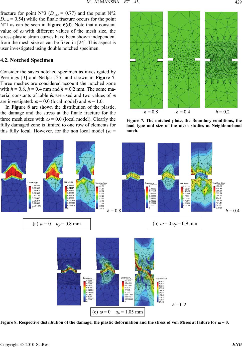

M. ALMANSBA ET AL.429
fracture for point N°3 (Dmax = 0.77) and the point N°2
Dmax = 0.54) while the finale fracture occurs for the point
N°1 as can be seen in Figure 6(d). Note that a constant
value of  with different values of the mesh size, the
stress-plastic strain curves have been shown independent
from the mesh size as can be fixed in [24]. This aspect is
user investigated using double notched specimen.
4.2. Notched Specimen
Consider the saves notched specimen as investigated by
Peerlings [3] and Nedjar [25] and shown in Figure 7.
Three meshes are considered account the notched zone
with h = 0.8, h = 0.4 mm and h = 0.2 mm. The some ma-
terial constants of table & are used and two values of 
are investigated:
 = 0.0 (local model) and  = 1.0.
In Figure 8 are shown the distribution of the plastic,
the damage and the stress at the finale fracture for the
three mesh sizes with  = 0.0 (local model). Clearly the
fully damaged zone is limited to one row of elements for
this fully local. However, for the non local model (  =
h = 0.8 h = 0.4 h = 0.2
Figure 7. The notched plate, the Boundary conditions, the
load type and size of the mesh studies at Neighbourhood
notch.
h = 0.8h = 0.4
(b)

= 0 ufr = 0.9 mm
(a)

= 0 ufr = 0.8 mm
h = 0.2
(c)
 = 0 ufr = 1.05 mm
Figure 8. Respective distribution of the damage, the plastic deformation and the stress of von Mises at failure for  = 0.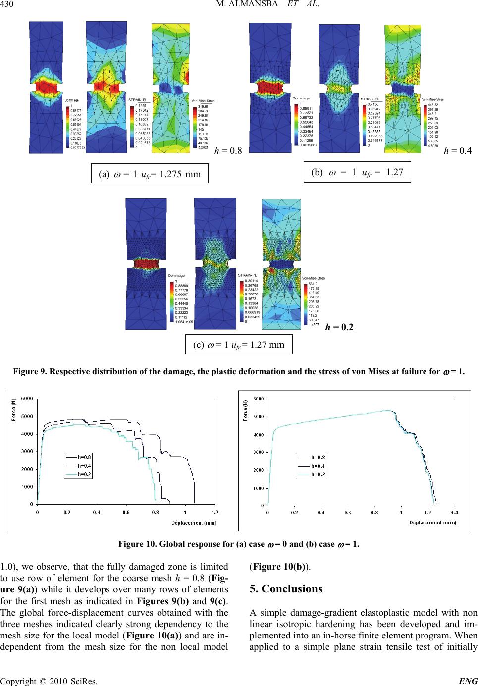

M. ALMANSBA ET AL. 430
h = 0.8 h = 0.4
h = 0.2
Figure 9. Respective distribution of the damage, the plastic deformation and the stress of von Mises at failure for  = 1.
Figure 10. Global response for (a) case  = 0 and (b) case  = 1.
1.0), we observe, that the fully damaged zone is limited
to use row of element for the coarse mesh h = 0.8 (Fig-
ure 9(a)) while it develops over many rows of elements
for the first mesh as indicated in Figures 9(b) and 9(c).
The global force-displacement curves obtained with the
three meshes indicated clearly strong dependency to the
mesh size for the local model (Figure 10(a)) and are in-
dependent from the mesh size for the non local model
(Figure 10(b)).
5. Conclusions
A simple damage-gradient elastoplastic model with non
linear isotropic hardening has been developed and im-
plemented into an in-horse finite element program. When
applied to a simple plane strain tensile test of initially
(
a
)

= 1 u
fr
= 1.275 m
m
(b)

= 1 u
fr
= 1.27
(
c
)

=1 u=1.27m
m
fr

M. ALMANSBA ET AL.431
homogeneous and initially notched specimen, the model
show a clear independence of the results on the mesh
size when the internal length scale is non zero. This
model will be implanted into a general propose Finite
elements program in order to show its ability to give a
mesh independent solution for more complex structures
as in metal forming. Also the extension to the 3D struc-
tures is under program.
6
. References
[1] G. Pijaudier-Cabot and Z. Bažant, “Nonlocal Continuum
Damage, Localization Instability and Convergence,” In-
ternational Journal of Applied Mechanics, Vol. 55, No. 4,
1988, pp. 287-293.
[2] K. Saanouni, “Sur l’Analyse de la Fissuration des Mili-
eux Elasto-Viscoplastique par la Théorie de l’Endom-
magement Continue,” Thèse de Doctorat, Université de
Technologie de Compiègne, 1988.
[3] T. Svedberg and K. Runesson, “An Adaptive Finite Ele-
ment Algorithm for Gradient Theory of Plasticity with
Coupling to Damage,” International Journal of Solids
Structures, Vol. 37, No. 48-50, 2000, pp. 7481-7499.
[4] R. H. J. Peerlings, “Enhanced Damage Modelling for
Fracture and Fatigue,” Ph.D. Dissertation, Technische
Universiteit Eindhoven, 1999.
[5] C. Comi, “A Nonlocal Model with Tension and Com-
pression Damage Mechanics,” European Journal of Me-
chanics A/Solids, Vol. 20, No. 1, 2001, pp. 1-22.
[6] M. Geers, R. Ubachs and R. Engelen, “Strongly Non-
Local Gradient-Enhanced Finit Strain Elastoplasticity,”
International Journal for Numerical Methods in Engin-
eering, Vol. 56, No. 14, 2003, pp. 2039-2068.
[7] R. Abu-Al-Rub and G. Voyiadjis, “A Physically Based
Gradient Plasticity Theory,” International Journal of
Plasticity, Vol. 22, No. 4, 2006, pp. 654-684.
[8] K. Saanouni and J.-L. Chaboche, “Comprehencive Struc-
tural Integrity,” Vol. 10, 2003.
[9] R. Mindlin and N. Eshel, “On First Strain Gradient Theo-
ries in Linear Elasticity,” International Journal of Solids
and Structures, Vol. 4, No. 1, 1968, pp. 109-124.
[10] P. Germain, “The Method of Virtual Power in Continuum
Mechanics, Part 2: Microstructure,” SIAM Journal on
Applied Mathematics, Vol. 25, No. 3, 1973, pp. 556-575.
[11] G. Maugin, “Nonlocal Theories or Gradient-Type Theo-
ries: A Matter of Convenience,” Archives of Mechanics,
Vol. 31, No. 1, 1979, pp. 15-26.
[12] S. Forest and R. Sievert, “Elastoviscoplastic Constitutive
Frameworks for Generalized Continua,” Acta Mechanica,
Vol. 160, No. 1, 2003, pp. 71-111.
[13] A. Eringen, “Microcontinuum Field Theories: Vol. I
Foundations and Solids; Vol. II Fluent Media,” Springer,
New York, 1999.
[14] R. Chambon, D. Caillerie and T. Matsuchima, “Plastic
Continuum with Microstructure, Local Second Gradient
Theories for Geomaterials,” International Journal of
Solids and Structures, Vol. 38, 2001, pp. 8503-8527.
[15] S. Forest, “Micromorphic Approach for Gradient Elastic-
ity, Viscoplasticity and Damage,” Journal of Engineering
Mechanics, Vol. 135, No. 3, 2009, pp. 117-131.
[16] R. Peerlings, T. Massart and M. Geers, “A Thermody-
namical Motivated Implicit Gradient Damage Framework
and its Application to Brick Masonry Cracking,” Com-
puter Methods in Applied Mechanics and Engineering,
Vol. 193, No. 30-32, 2004, pp. 3403-3417.
[17] K. Saanouni, C. Forster and F. Ben-Hatira, “On the Ane-
lastic Flow with Damage,” International Journal of
Damage Mechanics, Vol. 3, No. 2, 1994, pp. 140-169.
[18] K. Saanouni, H. Badreddine and M. Ajmal, “Advances in
Virtual Metal Forming Including the Ductile Damage
Occurrence: Application to 3D Sheet Metal Deep Draw-
ing,” Journal of Engineering Materials and Technology,
Vol. 130, No. 2, 2008, 1-11.
[19] D. Sornin, “Sur les Formulations Elastoplastiques Non
Locales en Gradient d’Endommagement,” Thèse de Doc-
torat, Université de Technologie de Troyes, 2007.
[20] S. Boers, P. Schreurs and M.Geers, “Operator-Split
Damage-Plasticity Applied to Groove Forming in Food
Can Lids,” International Journal of Solids and Structures,
Vol. 42, No. 14, 2005, pp. 4154-4178.
[21] A. Simone, G. Wells and L. Sluys, “From Continuous to
Discontinuous Failure in a Gradient-Enhanced Conti-
nuum Damage Model,” Computer Methods in Applied
Mechanics and Engineering, Vol. 192, No. 41, 2003, pp.
4581-4607.
[22] Y. Hammi, “Simulation Numérique de l’Endommagement
dans les Procédés de Mise en Forme,” Université de
Technologie de Compiègne, 2000.
[23] D. R. J. Owen and E. Hinton, “Finite Elements in Plastic-
ity, Theory and Practice,” Pineridge Press Limited, Swan-
sea, 1988.
[24] M. Almansba, K. Saanouni and N. E. Hannachi, “Régu-
larisation d'un Modèle Elastoplastique par Introduction
d'un Gradient d'endommagement,” XIXème Congrès Français
de Mécanique, CFM’09, France, 2009.
[25] B. Nedjar, “Elastoplastic-Damage Modelling Including
the Gradient of Damage: Formulation and Computational
Aspects,” International Journal of Solids and Structures,
Vol. 38, No. 30-31, 2001, pp. 5421-5451.