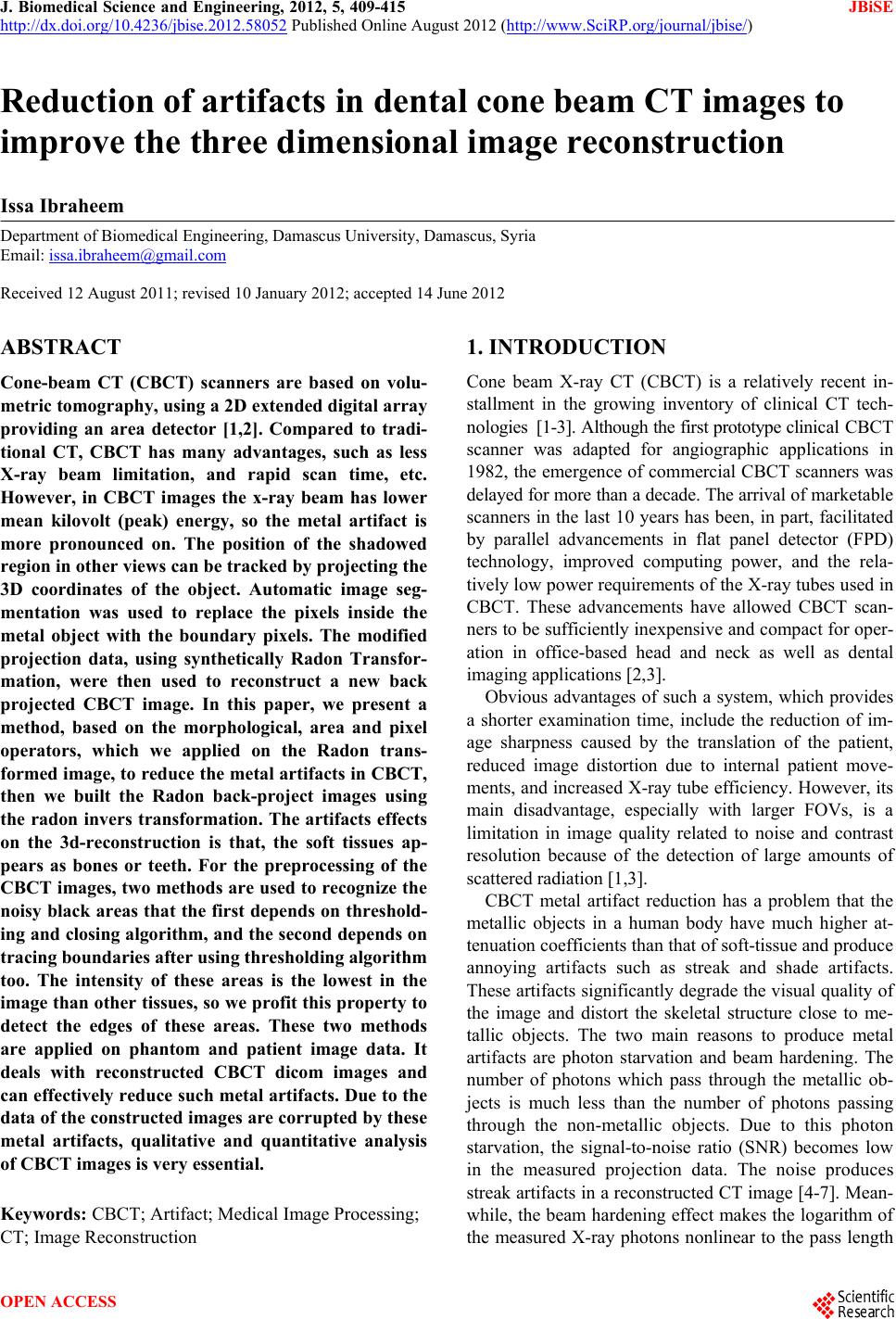
 J. Biomedical Science and Engineering, 2012, 5, 409-415 JBiSE http://dx.doi.org/10.4236/jbise.2012.58052 Published Online August 2012 (http://www.SciRP.org/journal/jbise/) Reduction of artifacts in dental cone beam CT images to improve the three dimensional image reconstruction Issa Ibraheem Department of Biomedical Engineering, Damascus University, Damascus, Syria Email: issa.ibraheem@gmail.com Received 12 August 2011; revised 10 January 2012; accepted 14 June 2012 ABSTRACT Cone-beam CT (CBCT) scanners are based on volu- metric tomography, using a 2D extended digital array providing an area detector [1,2]. Compared to tradi- tional CT, CBCT has many advantages, such as less X-ray beam limitation, and rapid scan time, etc. However, in CBCT images the x-ray beam has lower mean kilovolt (peak) energy, so the metal artifact is more pronounced on. The position of the shadowed region in other views can be tracked by projecting the 3D coordinates of the object. Automatic image seg- mentation was used to replace the pixels inside the metal object with the boundary pixels. The modified projection data, using synthetically Radon Transfor- mation, were then used to reconstruct a new back projected CBCT image. In this paper, we present a method, based on the morphological, area and pixel operators, which we applied on the Radon trans- formed image, to reduce the metal artifacts in CBCT, then we built the Radon back-project images using the radon invers transformation. The artifacts effects on the 3d-reconstruction is that, the soft tissues ap- pears as bones or teeth. For the preprocessing of the CBCT images, two methods are used to recognize the noisy black areas that the first depends on threshold- ing and closing algorithm, and the second depends on tracing boundaries after using thresholding algorithm too. The intensity of these areas is the lowest in the image than other tissues, so we profit this property to detect the edges of these areas. These two methods are applied on phantom and patient image data. It deals with reconstructed CBCT dicom images and can effectively reduce such metal artifacts. Due to the data of the constructed images are corrupted by these metal artifacts, qualitative and quantitative analysis of CBCT images is very essential. Keywords: CBCT; Artifact; Medical Image Processing; CT; Image Reconstruction 1. INTRODUCTION Cone beam X-ray CT (CBCT) is a relatively recent in- stallment in the growing inventory of clinical CT tech- nologies [1-3]. Although the first prototype clinical CBCT scanner was adapted for angiographic applications in 1982, the emergence of commercial CBCT scanners was delayed for more than a decade. The arrival of marketable scanners in the last 10 years has been, in part, facilitated by parallel advancements in flat panel detector (FPD) technology, improved computing power, and the rela- tively low power requirements of the X-ray tubes used in CBCT. These advancements have allowed CBCT scan- ners to be sufficiently inexpensive and compact for oper- ation in office-based head and neck as well as dental imaging applications [2,3]. Obvious advantages of such a system, which provides a shorter examination time, include the reduction of im- age sharpness caused by the translation of the patient, reduced image distortion due to internal patient move- ments, and increased X-ray tube efficiency. However, its main disadvantage, especially with larger FOVs, is a limitation in image quality related to noise and contrast resolution because of the detection of large amounts of scattered radiation [1,3]. CBCT metal artifact reduction has a problem that the metallic objects in a human body have much higher at- tenuation coefficients than that of soft-tissue and produce annoying artifacts such as streak and shade artifacts. These artifacts significantly degrade the visual quality of the image and distort the skeletal structure close to me- tallic objects. The two main reasons to produce metal artifacts are photon starvation and beam hardening. The number of photons which pass through the metallic ob- jects is much less than the number of photons passing through the non-metallic objects. Due to this photon starvation, the signal-to-noise ratio (SNR) becomes low in the measured projection data. The noise produces streak artifacts in a reconstructed CT image [4-7]. Mean- while, the beam hardening effect makes the logarithm of the measured X-ray photons nonlinear to the pass length OPEN ACCESS 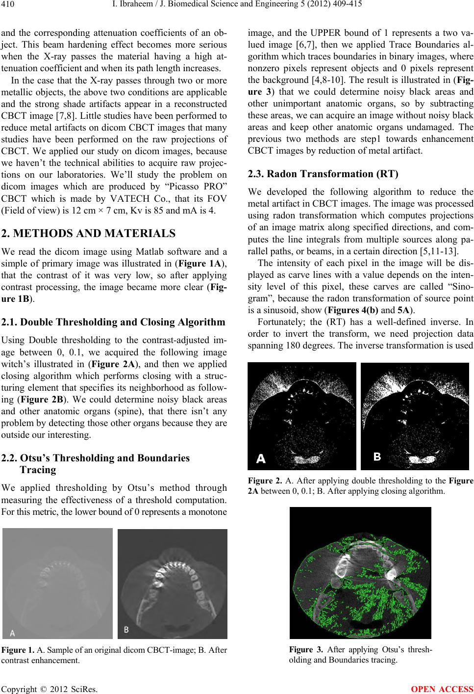 I. Ibraheem / J. Biomedical Science and Engineering 5 (2012) 409-415 410 and the corresponding attenuation coefficients of an ob- ject. This beam hardening effect becomes more serious when the X-ray passes the material having a high at- tenuation coefficient and when its path length increases. In the case that the X-ray passes through two or more metallic objects, the above two conditions are applicable and the strong shade artifacts appear in a reconstructed CBCT image [7,8]. Little studies have been performed to reduce metal artifacts on dicom CBCT images that many studies have been performed on the raw projections of CBCT. We applied our study on dicom images, because we haven’t the technical abilities to acquire raw projec- tions on our laboratories. We’ll study the problem on dicom images which are produced by “Picasso PRO” CBCT which is made by VATECH Co., that its FOV (Field of view) is 12 cm × 7 cm, Kv is 85 and mA is 4. 2. METHODS AND MATERIALS We read the dicom image using Matlab software and a simple of primary image was illustrated in (Figure 1A), that the contrast of it was very low, so after applying contrast processing, the image became more clear (Fig- ure 1B). 2.1. Double Thresholding and Closing Algorithm Using Double thresholding to the contrast-adjusted im- age between 0, 0.1, we acquired the following image witch’s illustrated in (Figure 2A), and then we applied closing algorithm which performs closing with a struc- turing element that specifies its neighborhood as follow- ing (Figure 2B). We could determine noisy black areas and other anatomic organs (spine), that there isn’t any problem by detecting those other organs because they are outside our interesting. 2.2. Otsu’s Thresholding and Boundaries Tracing We applied thresholding by Otsu’s method through measuring the effectiveness of a threshold computation. For this metric, the lower bound of 0 represents a monotone Figure 1. A. Sample of an original dicom CBCT-image; B. After contrast enhancement. image, and the UPPER bound of 1 represents a two va- lued image [6,7], then we applied Trace Boundaries al- gorithm which traces boundaries in binary images, where nonzero pixels represent objects and 0 pixels represent the background [4,8-10]. The result is illustrated in (Fig- ure 3) that we could determine noisy black areas and other unimportant anatomic organs, so by subtracting these areas, we can acquire an image without noisy black areas and keep other anatomic organs undamaged. The previous two methods are step1 towards enhancement CBCT images by reduction of metal artifact. 2.3. Radon Transformation (RT) We developed the following algorithm to reduce the metal artifact in CBCT images. The image was processed using radon transformation which computes projections of an image matrix along specified directions, and com- putes the line integrals from multiple sources along pa- rallel paths, or beams, in a certain direction [5,11-13]. The intensity of each pixel in the image will be dis- played as carve lines with a value depends on the inten- sity level of this pixel, these carves are called “Sino- gram”, because the radon transformation of source point is a sinusoid, show (Figures 4(b) and 5A). Fortunately; the (RT) has a well-defined inverse. In order to invert the transform, we need projection data spanning 180 degrees. The inverse transformation is used Figure 2. A. After applying double thresholding to the Figure 2A between 0, 0.1; B. After applying closing algorithm. Figure 3. After applying Otsu’s thresh- olding and Boundaries tracing. Copyright © 2012 SciRes. OPEN ACCESS 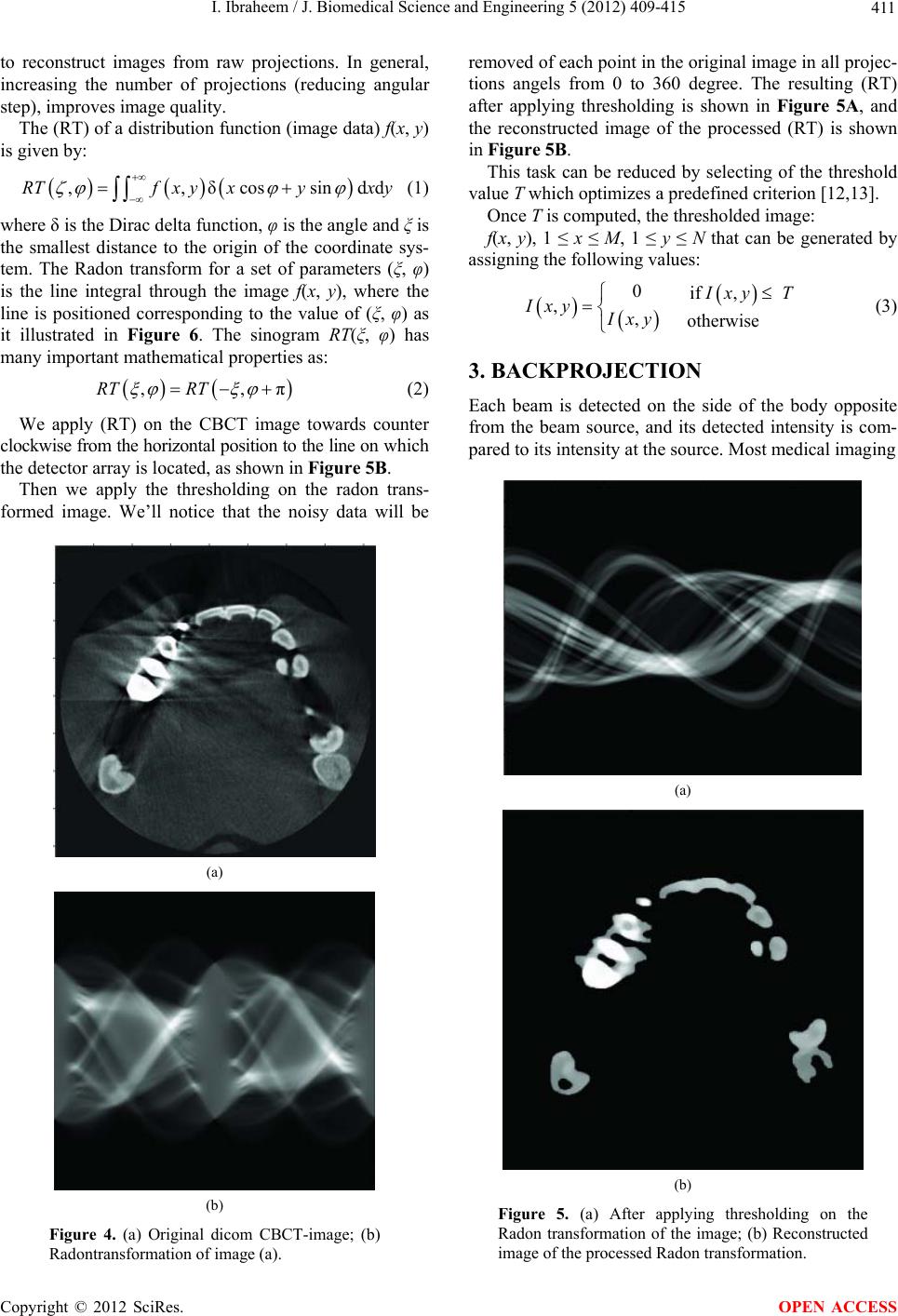 I. Ibraheem / J. Biomedical Science and Engineering 5 (2012) 409-415 411 to reconstruct images from raw projections. In general, increasing the number of projections (reducing angular step), improves image quality. The (RT) of a distribution function (image data) f(x, y) is given by: ,,δcossind dRTfx yxyx y (1) where δ is the Dirac delta function, φ is the angle and ξ is the smallest distance to the origin of the coordinate sys- tem. The Radon transform for a set of parameters (ξ, φ) is the line integral through the image f(x, y), where the line is positioned corresponding to the value of (ξ, φ) as it illustrated in Figure 6. The sinogram RT(ξ, φ) has many important mathematical properties as: ,,πRT RT (2) We apply (RT) on the CBCT image towards counter clockwise from the horizontal position to the line on which the detector array is located, as shown in Figure 5B. Then we apply the thresholding on the radon trans- formed image. We’ll notice that the noisy data will be (a) (b) Figure 4. (a) Original dicom CBCT-image; (b) Radontransformation of image (a). removed of each point in the original image in all projec- tions angels from 0 to 360 degree. The resulting (RT) after applying thresholding is shown in Figure 5A, and the reconstructed image of the processed (RT) is shown in Figure 5B. This task can be reduced by selecting of the threshold value T which optimizes a predefined criterion [12,13]. Once T is computed, the thresholded image: f(x, y), 1 ≤ x ≤ M, 1 ≤ y ≤ N that can be generated by assigning the following values: 0if , , , otherwise xy T Ixy Ixy (3) 3. BACKPROJECTION Each beam is detected on the side of the body opposite from the beam source, and its detected intensity is com- pared to its intensity at the source. Most medical imaging (a) (b) Figure 5. (a) After applying thresholding on the Radon transformation of the image; (b) Reconstructed image of the processed Radon transformation. Copyright © 2012 SciRes. OPEN ACCESS 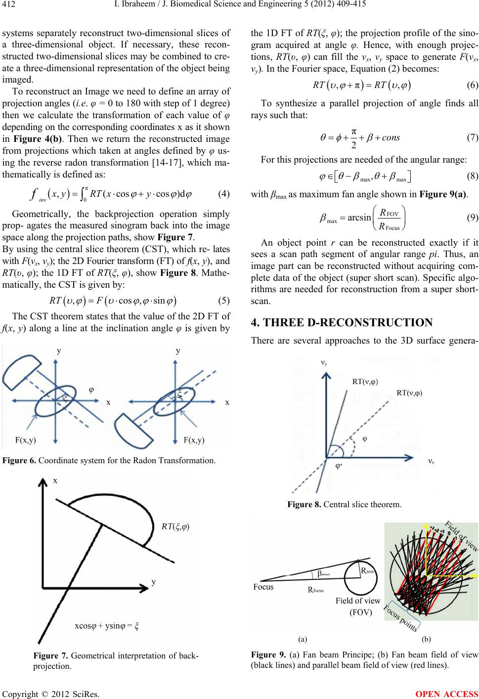 I. Ibraheem / J. Biomedical Science and Engineering 5 (2012) 409-415 412 systems separately reconstruct two-dimensional slices of a three-dimensional object. If necessary, these recon- structed two-dimensional slices may be combined to cre- ate a three-dimensional representation of the object being imaged. To reconstruct an Image we need to define an array of projection angles (i.e. φ = 0 to 180 with step of 1 degree) then we calculate the transformation of each value of φ depending on the corresponding coordinates x as it shown in Figure 4(b). Then we return the reconstructed image from projections which taken at angles defined by φ us- ing the reverse radon transformation [14-17], which ma- thematically is defined as: π 0 ,(coscos inv xy RTxy f)d (4) Geometrically, the backprojection operation simply prop- agates the measured sinogram back into the image space along the projection paths, show Figure 7. By using the central slice theorem (CST), which re- lates with F(νx, νy); the 2D Fourier transform (FT) of f(x, y), and RT(υ, φ); the 1D FT of RT(ξ, φ), show Figure 8. Mathe- matically, the CST is given by: ,cos,siRT F n (5) The CST theorem states that the value of the 2D FT of f(x, y) along a line at the inclination angle φ is given by Figure 6. Coordinate system for the Radon Transformation. Figure 7. Geometrical interpretation of back- projection. the 1D FT of RT(ξ, φ); the projection profile of the sino- gram acquired at angle φ. Hence, with enough projec- tions, RT(υ, φ) can fill the νx, νy space to generate F(νx, νy). In the Fourier space, Equation (2) becomes: ,π,RT RT (6) To synthesize a parallel projection of angle finds all rays such that: π 2cons (7) For this projections are needed of the angular range: max max , (8) with βmax as maximum fan angle shown in Figure 9(a). FOV max Focu s arcsin R R (9) An object point r can be reconstructed exactly if it sees a scan path segment of angular range pi. Thus, an image part can be reconstructed without acquiring com- plete data of the object (super short scan). Specific algo- rithms are needed for reconstruction from a super short- scan. 4. THREE D-RECONSTRUCTION There are several approaches to the 3D surface genera- Figure 8. Central slice theorem. (a) (b) Figure 9. (a) Fan beam Principe; (b) Fan beam field of view (black lines) and parallel beam field of view (red lines). Copyright © 2012 SciRes. OPEN ACCESS 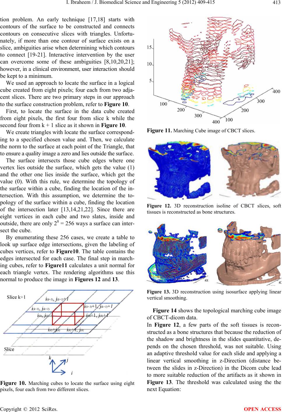 I. Ibraheem / J. Biomedical Science and Engineering 5 (2012) 409-415 413 tion problem. An early technique [17,18] starts with contours of the surface to be constructed and connects contours on consecutive slices with triangles. Unfortu- nately, if more than one contour of surface exists on a slice, ambiguities arise when determining which contours to connect [19-21]. Interactive intervention by the user can overcome some of these ambiguities [8,10,20,21]; however, in a clinical environment, user interaction should be kept to a minimum. We used an approach to locate the surface in a logical cube created from eight pixels; four each from two adja- cent slices. There are two primary steps in our approach to the surface construction problem, refer to Figure 10. First, to locate the surface in the data cube created from eight pixels, the first four from slice k while the second four from k + 1 slice as it shown in Figure 10. We create triangles with locate the surface correspond- ing to a specified chosen value and. Then, we calculate the norm to the surface at each point of the Triangle, that to ensure a quality image a zero and lies outside the surface. The surface intersects those cube edges where one vertex lies outside the surface, which gets the value (1) and the other one lies inside the surface, which get the value (0). With this rule, we determine the topology of the surface within a cube, finding the location of the in- tersection. With this assumption, we determine the to- pology of the surface within a cube, finding the location of the intersection later [13,14,21,22]. Since there are eight vertices in each cube and two slates, inside and outside, there are only 28 = 256 ways a surface can inter- sect the cube. By enumerating these 256 cases, we create a table to look up surface edge intersections, given the labeling of cubes vertices, refer to Figure10. The table contains the edges intersected for each case. The final step in march- ing cubes, refer to Figure11 calculates a unit normal for each triangle vertex. The rendering algorithms use this normal to produce the image in Figures 12 and 13. Figure 10. Marching cubes to locate the surface using eight pixels, four each from two different slices. Figure 11. Marching Cube image of CBCT slices. Figure 12. 3D reconstruction isoline of CBCT slices, soft tissues is reconstructed as bone structures. Figure 13. 3D reconstruction using isosurface applying linear vertical smoothing. Figure 14 shows the topological marching cube image of CBCT-dicom data. In Figure 12, a few parts of the soft tissues is recon- structed as a bone structures that because the reduction of the shadow and brightness in the slides quantitative, de- pends on the chosen threshold, was not suitable. Using an adaptive threshold value for each slide and applying a linear vertical smoothing in z-Direction (distance be- tween the slides in z-Direction) in the Dicom cube lead to more suitable reduction of the artifacts as it shown in Figure 13. The threshold was calculated using the the next Equation: Copyright © 2012 SciRes. OPEN ACCESS 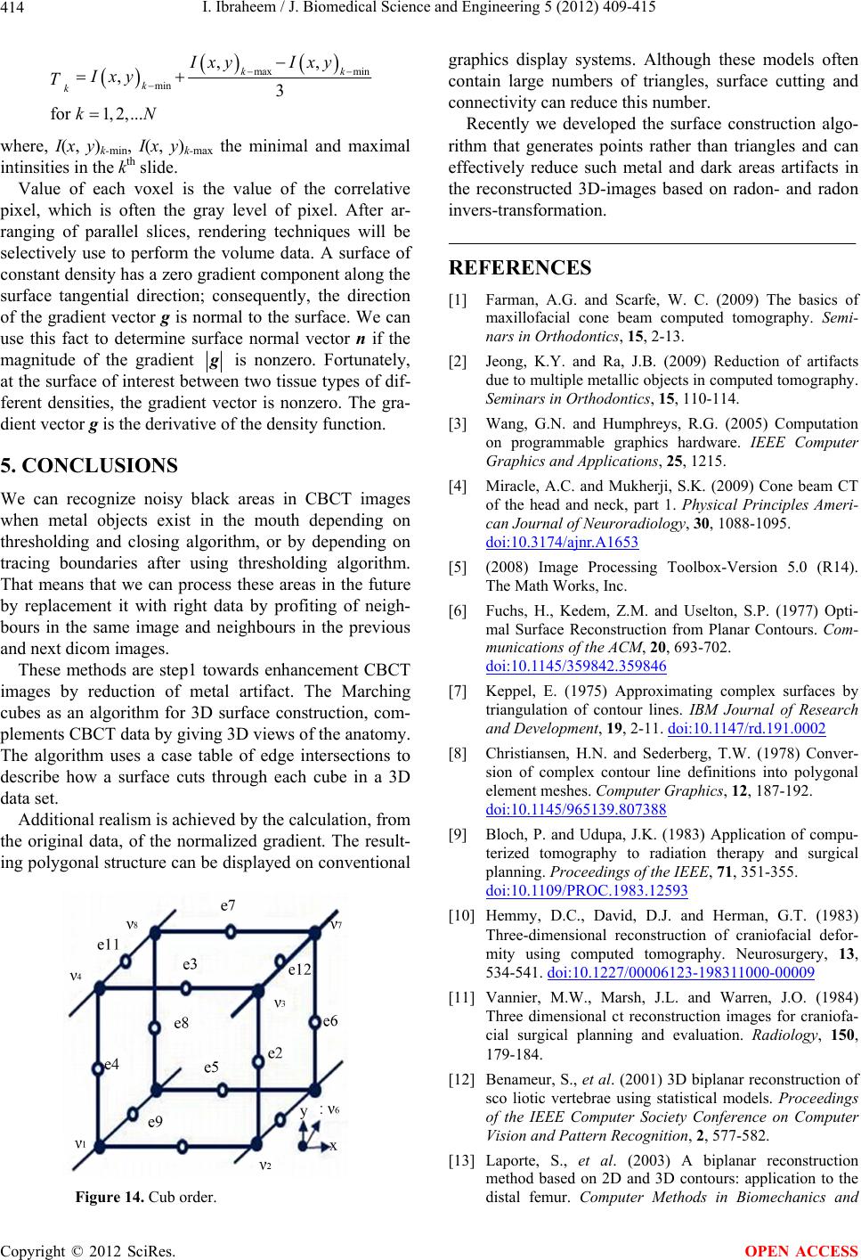 I. Ibraheem / J. Biomedical Science and Engineering 5 (2012) 409-415 414 max min min ,, ,3 for1, 2,... kk k k Ixy Ixy Ixy T kN where, I(x, y)k-min, I(x, y)k-max the minimal and maximal intinsities in the kth slide. Value of each voxel is the value of the correlative pixel, which is often the gray level of pixel. After ar- ranging of parallel slices, rendering techniques will be selectively use to perform the volume data. A surface of constant density has a zero gradient component along the surface tangential direction; consequently, the direction of the gradient vector g is normal to the surface. We can use this fact to determine surface normal vector n if the magnitude of the gradient g is nonzero. Fortunately, at the surface of interest between two tissue types of dif- ferent densities, the gradient vector is nonzero. The gra- dient vector g is the derivative of the density function. 5. CONCLUSIONS We can recognize noisy black areas in CBCT images when metal objects exist in the mouth depending on thresholding and closing algorithm, or by depending on tracing boundaries after using thresholding algorithm. That means that we can process these areas in the future by replacement it with right data by profiting of neigh- bours in the same image and neighbours in the previous and next dicom images. These methods are step1 towards enhancement CBCT images by reduction of metal artifact. The Marching cubes as an algorithm for 3D surface construction, com- plements CBCT data by giving 3D views of the anatomy. The algorithm uses a case table of edge intersections to describe how a surface cuts through each cube in a 3D data set. Additional realism is achieved by the calculation, from the original data, of the normalized gradient. The result- ing polygonal structure can be displayed on conventional Figure 14. Cub order. graphics display systems. Although these models often contain large numbers of triangles, surface cutting and connectivity can reduce this number. Recently we developed the surface construction algo- rithm that generates points rather than triangles and can effectively reduce such metal and dark areas artifacts in the reconstructed 3D-images based on radon- and radon invers-transformation. REFERENCES [1] Farman, A.G. and Scarfe, W. C. (2009) The basics of maxillofacial cone beam computed tomography. Semi- nars in Orthodontics, 15, 2-13. [2] Jeong, K.Y. and Ra, J.B. (2009) Reduction of artifacts due to multiple metallic objects in computed tomography. Seminars in Orthodontics, 15, 110-114. [3] Wang, G.N. and Humphreys, R.G. (2005) Computation on programmable graphics hardware. IEEE Computer Graphics and Applications, 25, 1215. [4] Miracle, A.C. and Mukherji, S.K. (2009) Cone beam CT of the head and neck, part 1. Physical Principles Ameri- can Journal of Neuroradiology, 30, 1088-1095. doi:10.3174/ajnr.A1653 [5] (2008) Image Processing Toolbox-Version 5.0 (R14). The Math Works, Inc. [6] Fuchs, H., Kedem, Z.M. and Uselton, S.P. (1977) Opti- mal Surface Reconstruction from Planar Contours. Com- munications of the ACM, 20, 693-702. doi:10.1145/359842.359846 [7] Keppel, E. (1975) Approximating complex surfaces by triangulation of contour lines. IBM Journal of Research and Development, 19, 2-11. doi:10.1147/rd.191.0002 [8] Christiansen, H.N. and Sederberg, T.W. (1978) Conver- sion of complex contour line definitions into polygonal element meshes. Computer Graphics, 12, 187-192. doi:10.1145/965139.807388 [9] Bloch, P. and Udupa, J.K. (1983) Application of compu- terized tomography to radiation therapy and surgical planning. Proceedings of the IEEE, 71, 351-355. doi:10.1109/PROC.1983.12593 [10] Hemmy, D.C., David, D.J. and Herman, G.T. (1983) Three-dimensional reconstruction of craniofacial defor- mity using computed tomography. Neurosurgery, 13, 534-541. doi:10.1227/00006123-198311000-00009 [11] Vannier, M.W., Marsh, J.L. and Warren, J.O. (1984) Three dimensional ct reconstruction images for craniofa- cial surgical planning and evaluation. Radiology, 150, 179-184. [12] Benameur, S., et al. (2001) 3D biplanar reconstruction of sco liotic vertebrae using statistical models. Proceedings of the IEEE Computer Society Conference on Computer Vision and Pattern Recognition, 2, 577-582. [13] Laporte, S., et al. (2003) A biplanar reconstruction method based on 2D and 3D contours: application to the distal femur. Computer Methods in Biomechanics and Copyright © 2012 SciRes. OPEN ACCESS 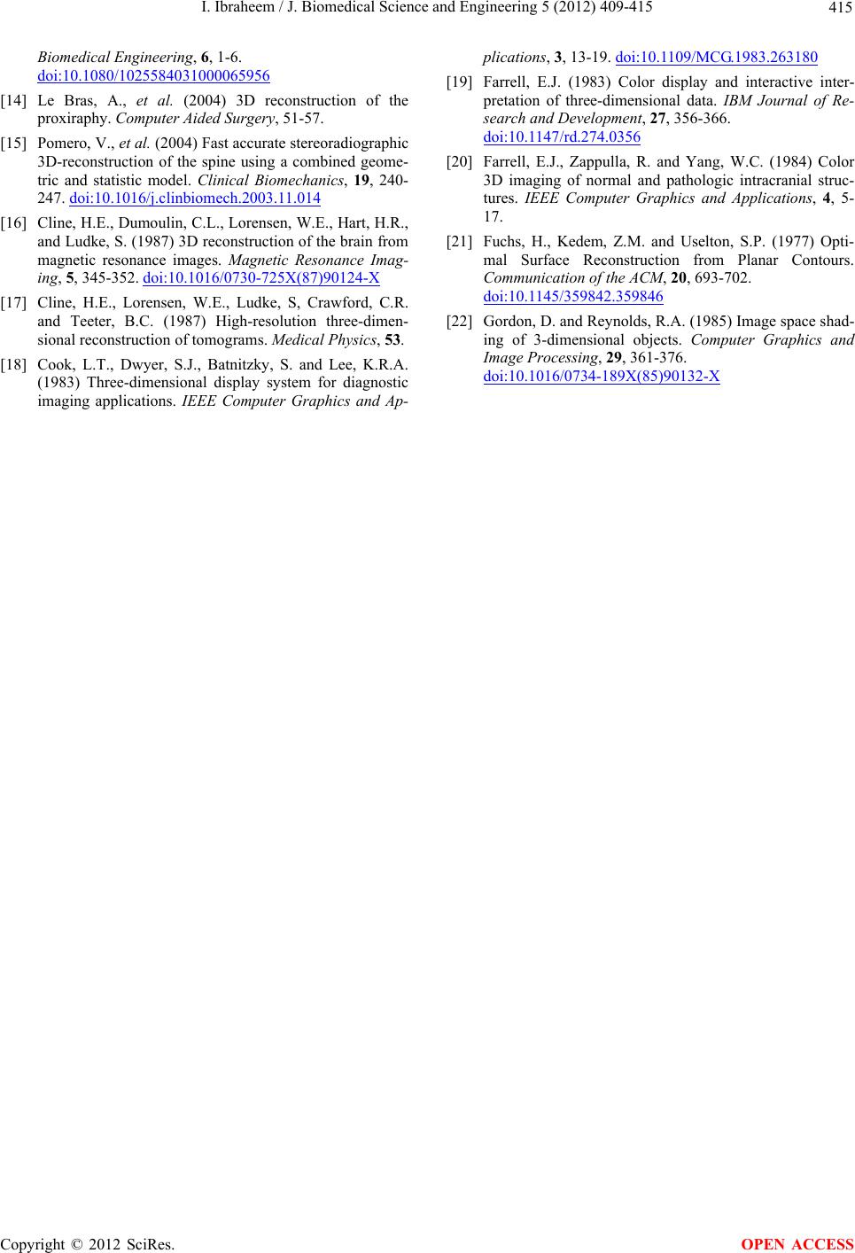 I. Ibraheem / J. Biomedical Science and Engineering 5 (2012) 409-415 Copyright © 2012 SciRes. 415 OPEN ACCESS Biomedical Engineering, 6, 1-6. doi:10.1080/1025584031000065956 [14] Le Bras, A., et al. (2004) 3D reconstruction of the proxiraphy. Computer Aided Surgery, 51-57. [15] Pomero, V., et al. (2004) Fast accurate stereoradiographic 3D-reconstruction of the spine using a combined geome- tric and statistic model. Clinical Biomechanics, 19, 240- 247. doi:10.1016/j.clinbiomech.2003.11.014 [16] Cline, H.E., Dumoulin, C.L., Lorensen, W.E., Hart, H.R., and Ludke, S. (1987) 3D reconstruction of the brain from magnetic resonance images. Magnetic Resonance Imag- ing, 5, 345-352. doi:10.1016/0730-725X(87)90124-X [17] Cline, H.E., Lorensen, W.E., Ludke, S, Crawford, C.R. and Teeter, B.C. (1987) High-resolution three-dimen- sional reconstruction of tomograms. Medical Physics, 53. [18] Cook, L.T., Dwyer, S.J., Batnitzky, S. and Lee, K.R.A. (1983) Three-dimensional display system for diagnostic imaging applications. IEEE Computer Graphics and Ap- plications, 3, 13-19. doi:10.1109/MCG.1983.263180 [19] Farrell, E.J. (1983) Color display and interactive inter- pretation of three-dimensional data. IBM Journal of Re- search and Development, 27, 356-366. doi:10.1147/rd.274.0356 [20] Farrell, E.J., Zappulla, R. and Yang, W.C. (1984) Color 3D imaging of normal and pathologic intracranial struc- tures. IEEE Computer Graphics and Applications, 4, 5- 17. [21] Fuchs, H., Kedem, Z.M. and Uselton, S.P. (1977) Opti- mal Surface Reconstruction from Planar Contours. Communication of the ACM, 20, 693-702. doi:10.1145/359842.359846 [22] Gordon, D. and Reynolds, R.A. (1985) Image space shad- ing of 3-dimensional objects. Computer Graphics and Image Processing, 29, 361-376. doi:10.1016/0734-189X(85)90132-X
|