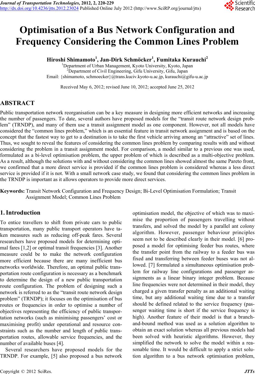
 Journal of Transportation Technologies, 2012, 2, 220-229 http://dx.doi.org/10.4236/jtts.2012.23024 Published Online July 2012 (http://www.SciRP.org/journal/jtts) Optimisation of a Bus Network Configuration and Frequency Considering the Common Lines Problem Hiroshi Shimamoto1, Jan-Dirk Schmöcker1, Fumitaka Kurauchi2 1Department of Urban Management, Kyoto University, Kyoto, Japan 2Department of Civil Engineering, Gifu University, Gifu, Japan Email: {shimamoto, schmoecker}@trans.kuciv.kyoto-u.ac.jp, kurauchi@gifu-u.ac.jp Received May 6, 2012; revised June 10, 2012; accepted June 25, 2012 ABSTRACT Public transportation network reorganisation can be a key measure in designing more efficient networks and increasing the number of passengers. To date, several authors have proposed models for the “transit route network design prob- lem” (TRNDP), and many of them use a transit assignment model as one component. However, not all models have considered the “common lines problem,” which is an essential feature in transit network assignment and is based on the concept that the fastest way to get to a destination is to take the first vehicle arriving among an “attractive” set of lines. Thus, we sought to reveal the features of considering the common lines problem by comparing results with and without considering the problem in a transit assignment model. For comparison, a model similar to a previous one was used, formulated as a bi-level optimisation problem, the upper problem of which is described as a multi-objective problem. As a result, although the solutions with and without considering the common lines showed almost the same Pareto front, we confirmed that a more direct service is provided if the common lines problem is considered whereas a less direct service is provided if it is not. With a small network case study, we found that considering the common lines problem in the TRNDP is important as it allows operators to provide more direct services. Keywords: Transit Network Configuration and Frequency Design; Bi-Level Optimisation Formulation; Transit Assignment Model; Common Lines Problem 1. Introduction To entice travellers to shift from private cars to public transportation, many public transport operators have ta- ken measures such as reducing off-peak fares. Several researchers have proposed models for determining opti- mal fares [1,2] or optimal transit frequencies [3]. Another measure could be to make the network configuration more efficient because there are many inefficient bus networks worldwide. Therefore, an optimal public trans- portation route configuration is necessary as a benchmark to determine the design of a new public transportation route configuration. The problem of designing such a network is referred to as the “transit route network design problem” (TRNDP); it focuses on the optimisation of bus routes or frequencies in order to optimise a number of objectives representing the efficiency of public transpor- tation networks (such as minimising passengers’ cost or maximising profit) under operational and resource con- straints such as the number and length of public trans- portation routes, allowable service frequencies, and the number of available buses [4]. Several researchers have proposed models for the TRNDP. For example, [5] also proposed a bus network optimisation model, the objective of which was to maxi- mise the proportion of passengers travelling without transfers, and solved the model by a parallel ant colony algorithm. However, passenger behaviour principles seem not to be described clearly in their model. [6] pro- posed a model for optimising feeder bus routes, where the transfer point from the railway to a feeder bus was fixed and transferring between feeder buses was not al- lowed. [7] formulated a simultaneous optimisation prob- lem for railway line configurations and passenger as- signments as a linear binary integer problem. Because line frequencies were not determined in their model, they charged a given transfer penalty as an additional waiting time, but any additional waiting time due to a transfer should be defined related to the service frequency (pas- senger waiting time is short if the service frequency is high). Another feature of their model is that a branch- and-bound method was used as a solution algorithm to obtain an exact solution whereas all previous models had been solved with heuristic algorithms. However, they simplified the network to solve the model within a rea- sonable time. It would be difficult to apply a strict solu- tion algorithm to a bus network optimisation problem, C opyright © 2012 SciRes. JTTs 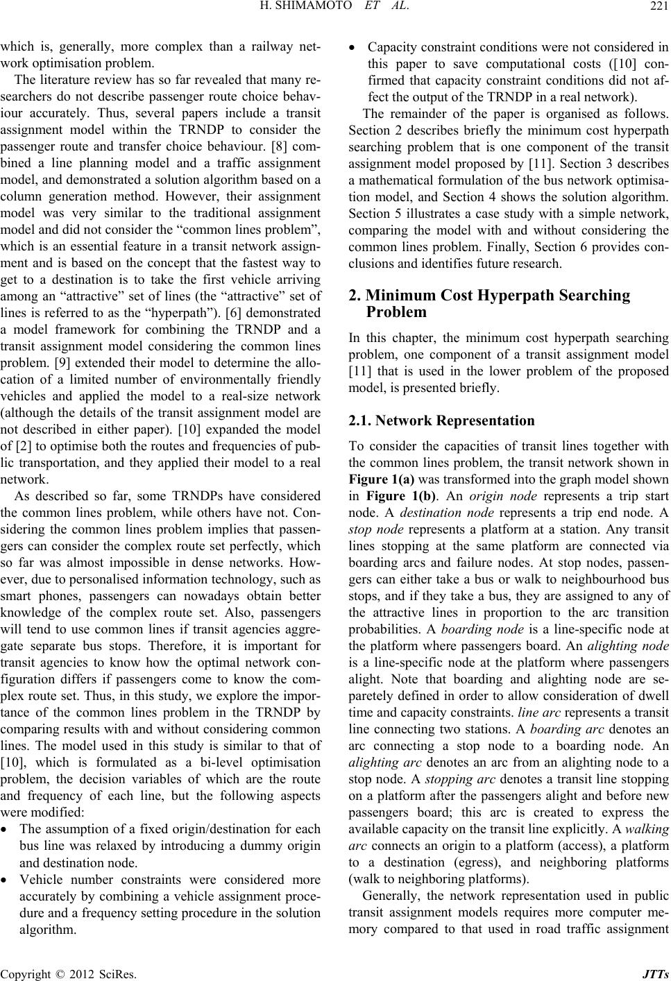 H. SHIMAMOTO ET AL. 221 which is, generally, more complex than a railway net- work optimisation problem. The literature review has so far revealed that many re- searchers do not describe passenger route choice behav- iour accurately. Thus, several papers include a transit assignment model within the TRNDP to consider the passenger route and transfer choice behaviour. [8] com- bined a line planning model and a traffic assignment model, and demonstrated a solution algorithm based on a column generation method. However, their assignment model was very similar to the traditional assignment model and did not consider the “common lines problem”, which is an essential feature in a transit network assign- ment and is based on the concept that the fastest way to get to a destination is to take the first vehicle arriving among an “attractive” set of lines (the “attractive” set of lines is referred to as the “hyperpath”). [6] demonstrated a model framework for combining the TRNDP and a transit assignment model considering the common lines problem. [9] extended their model to determine the allo- cation of a limited number of environmentally friendly vehicles and applied the model to a real-size network (although the details of the transit assignment model are not described in either paper). [10] expanded the model of [2] to optimise both the routes and frequencies of pub- lic transportation, and they applied their model to a real network. As described so far, some TRNDPs have considered the common lines problem, while others have not. Con- sidering the common lines problem implies that passen- gers can consider the complex route set perfectly, which so far was almost impossible in dense networks. How- ever, due to personalised information technology, such as smart phones, passengers can nowadays obtain better knowledge of the complex route set. Also, passengers will tend to use common lines if transit agencies aggre- gate separate bus stops. Therefore, it is important for transit agencies to know how the optimal network con- figuration differs if passengers come to know the com- plex route set. Thus, in this study, we explore the impor- tance of the common lines problem in the TRNDP by comparing results with and without considering common lines. The model used in this study is similar to that of [10], which is formulated as a bi-level optimisation problem, the decision variables of which are the route and frequency of each line, but the following aspects were modified: The assumption of a fixed origin/destination for each bus line was relaxed by introducing a dummy origin and destination node. Vehicle number constraints were considered more accurately by combining a vehicle assignment proce- dure and a frequency setting procedure in the solution algorithm. Capacity constraint conditions were not considered in this paper to save computational costs ([10] con- firmed that capacity constraint conditions did not af- fect the output of the TRNDP in a real network). The remainder of the paper is organised as follows. Section 2 describes briefly the minimum cost hyperpath searching problem that is one component of the transit assignment model proposed by [11]. Section 3 describes a mathematical formulation of the bus network optimisa- tion model, and Section 4 shows the solution algorithm. Section 5 illustrates a case study with a simple network, comparing the model with and without considering the common lines problem. Finally, Section 6 provides con- clusions and identifies future research. 2. Minimum Cost Hyperpath Searching Problem In this chapter, the minimum cost hyperpath searching problem, one component of a transit assignment model [11] that is used in the lower problem of the proposed model, is presented briefly. 2.1. Network Representation To consider the capacities of transit lines together with the common lines problem, the transit network shown in Figure 1(a) was transformed into the graph model shown in Figure 1(b). An origin node represents a trip start node. A destination node represents a trip end node. A stop node represents a platform at a station. Any transit lines stopping at the same platform are connected via boarding arcs and failure nodes. At stop nodes, passen- gers can either take a bus or walk to neighbourhood bus stops, and if they take a bus, they are assigned to any of the attractive lines in proportion to the arc transition probabilities. A boarding node is a line-specific node at the platform where passengers board. An alighting node is a line-specific node at the platform where passengers alight. Note that boarding and alighting node are se- paretely defined in order to allow consideration of dwell time and capacity constraints. line arc represents a transit line connecting two stations. A boarding arc denotes an arc connecting a stop node to a boarding node. An alighting arc denotes an arc from an alighting node to a stop node. A stopping arc denotes a transit line stopping on a platform after the passengers alight and before new passengers board; this arc is created to express the available capacity on the transit line explicitly. A walking arc connects an origin to a platform (access), a platform to a destination (egress), and neighboring platforms (walk to neighboring platforms). Generally, the network representation used in public transit assignment models requires more computer me- mory compared to that used in road traffic assignment Copyright © 2012 SciRes. JTTs 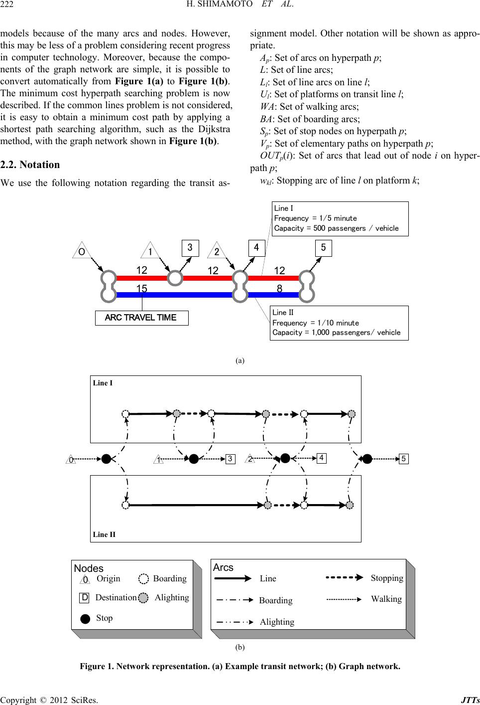 H. SHIMAMOTO ET AL. Copyright © 2012 SciRes. JTTs 222 models because of the many arcs and nodes. However, this may be less of a problem considering recent progress in computer technology. Moreover, because the compo- nents of the graph network are simple, it is possible to convert automatically from Figure 1(a) to Figure 1(b). The minimum cost hyperpath searching problem is now described. If the common lines problem is not considered, it is easy to obtain a minimum cost path by applying a shortest path searching algorithm, such as the Dijkstra method, with the graph network shown in Figure 1(b). 2.2. Notation We use the following notation regarding the transit as- signment model. Other notation will be shown as appro- priate. Ap: Set of arcs on hyperpath p; L: Set of line arcs; Ll: Set of line arcs on line l; Ul: Set of platforms on transit line l; WA: Set of walking arcs; BA: Set of boarding arcs; Sp: Set of stop nodes on hyperpath p; Vp: Set of elementary paths on hyperpath p; OUTp(i): Set of arcs that lead out of node i on hyper- path p; wkl: Stopping arc of line l on platform k; O1 2 3 45 Line I Frequency = 1/5 minute Capacity = 500 passengers / vehicle Line II Frequency = 1/10 minute Capacity = 1,000 passengers/ vehicle 12 12 12 15 8 ARC TRAVEL TIME (a) Nodes 0 D Origin Destination Stop Boarding Alighting Arcs Line Boarding Alighting Stopping Walking Line II Line I 4 253 10 (b) Figure 1. Network representation. (a) Example transit network; (b) Graph network. 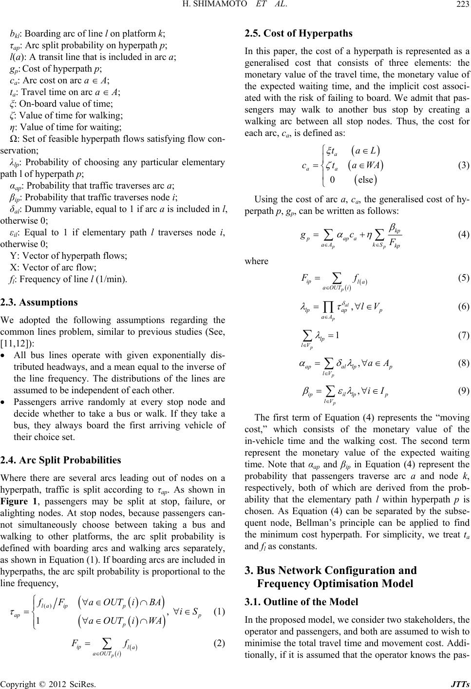 H. SHIMAMOTO ET AL. 223 bkl: Boarding arc of line l on platform k; ; ; lows satisfying flow con- se cluded in l, ot 2.3. Assum lowing assumptions regarding the es ading out of nodes on a τap: Arc split probability on hyperpath p; l(a): A transit line that is included in arc a gp: Cost of hyperpath p; ; ca: Arc cost on arc a A ta: Travel time on arc a A ξ: On-board value of time; ;ζ: Value of time for walking η: Value of time for waiting; Ω: Set of feasible hyperpath f rvation; λlp: Probability of choosing any particular elementary path l of hyperpath p; αap: Probability that traffic traverses arc a; βip: Probability that traffic traverses node i; δal: Dummy variable, equal to 1 if arc a is in herwise 0; εil: Equal to 1 if elementary path l traverses node i, otherwise 0; Y: Vector of hyperpath flows; X: Vector of arc flow; /min). fl: Frequency of line l (1 ptions We adopted the fol common lines problem, similar to previous studies (See, [11,12]): All bus lines operate with given exponentially dis- tributed headways, and a mean equal to the inverse of the line frequency. The distributions of the lines are assumed to be independent of each other. Passengers arrive randomly at every stop node and decide whether to take a bus or walk. If they take a bus, they always board the first arriving vehicle of their choice set. 2.4. Arc Split Probabiliti Where there are several arcs le hyperpath, traffic is split according to τap. As shown in Figure 1, passengers may be split at stop, failure, or alighting nodes. At stop nodes, because passengers can- not simultaneously choose between taking a bus and walking to other platforms, the arc split probability is defined with boarding arcs and walking arcs separately, as shown in Equation (1). If boarding arcs are included in hyperpaths, the arc spilt probability is proportional to the line frequency, () , 1 la ipp ap p p f F aOUT iBA iS aOUT iWA (1) (2) 2.5. Cost of Hyperpaths In this paper, the cost of a hyperpa generalised cost that consists of three elements: the time, the monetary value of th is represented as a p ip la a OUTi f monetary value of the travel the expected waiting time, and the implicit cost associ- ated with the risk of failing to board. We admit that pas- sengers may walk to another bus stop by creating a walking arc between all stop nodes. Thus, the cost for each arc, ca, is defined as: 0 a aa taL ctaWA (3) else Using the cost of arc a, ca, the generalised cost of hy- perpath p, gp, can be written as follows: pp pa pa aAkS kp gc kp (4) where p ip la aOUT i f (5) , al p lp app aA lV (6) 1 p lp lV (7) , p apal lpp lV aA (8) , p ipil lpp lV iI (9) The first term of Equation (4) represents the “moving cost,” which consists of the mon in-vehicle time and the walking co represen 3.1. Outline of the Model olders, the oped to wish to and movement cost. Addi- he operator knows the pas- etary value of the st. The second term t the monetary value of the expected waiting time. Note that αap and βip in Equation (4) represent the probability that passengers traverse arc a and node k, respectively, both of which are derived from the prob- ability that the elementary path l within hyperpath p is chosen. As Equation (4) can be separated by the subse- quent node, Bellman’s principle can be applied to find the minimum cost hyperpath. For simplicity, we treat ta and fl as constants. 3. Bus Network Configuration and Frequency Optimisation Model In the proposed model, we consider two stakeh erator and passengers, and both are assum minimise the total travel time tionally, if it is assumed that t Copyright © 2012 SciRes. JTTs 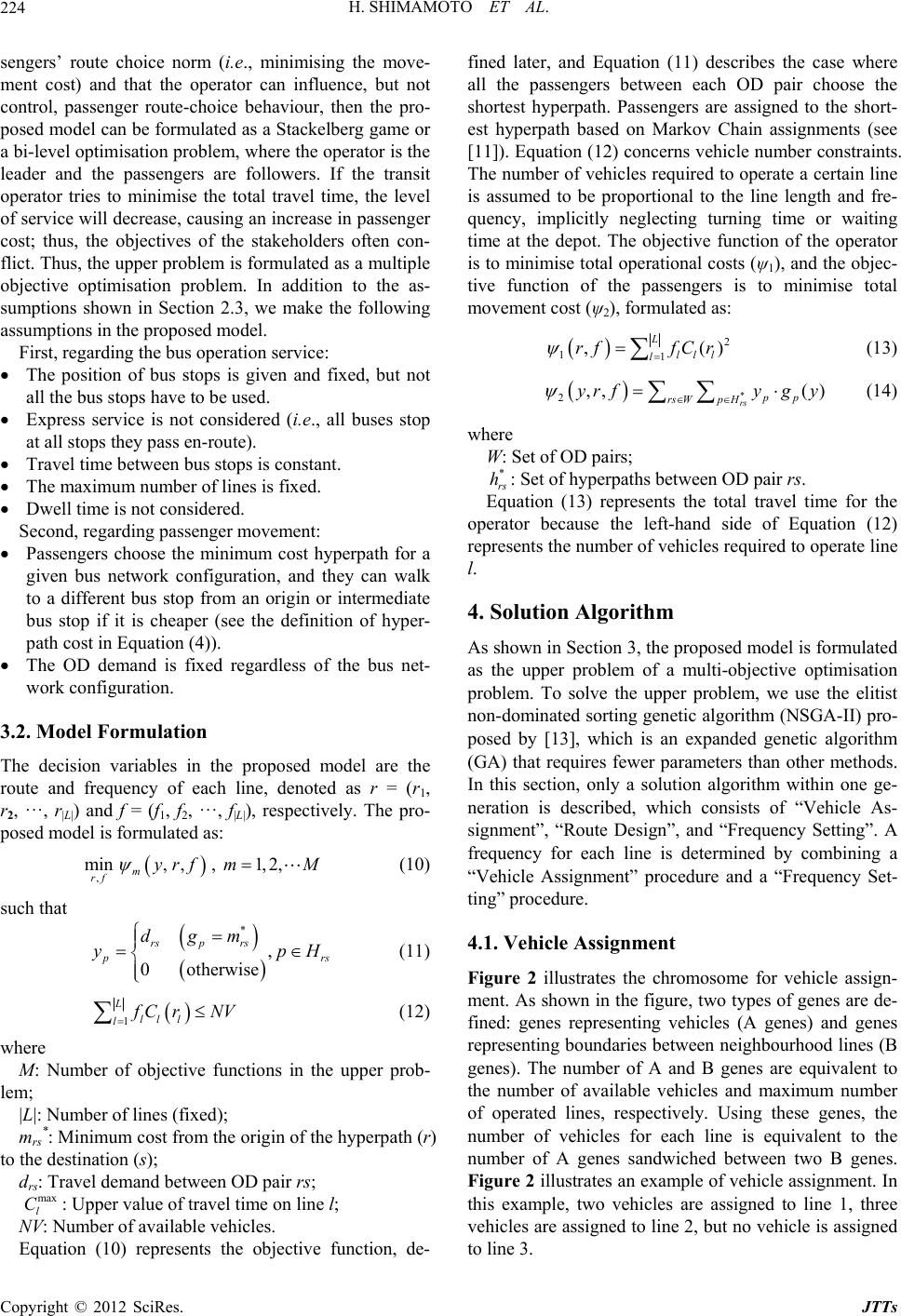 H. SHIMAMOTO ET AL. 224 sengers’ route choice norm (i.e., minimising the move- ment cost) and that the operator can influence, but not control, passenger route-choice behaviour, then the pro- posed model can be formulated as a Stackelberg game or a bi-level optimisation problem, where the operator is the leader and the passengers are followers. If the transit operator tries to minimise the total travel time, the level of service will decrease, causing an increase in passenger cost; thus, the objectives of the stakeholders often con- flict. Thus, the upper problem is formulated as a multiple objective optimisation problem. In addition to the as- sumptions shown in Section 2.3, we make the following assumptions in the proposed model. First, regarding the bus operation service: The position of bus stops is given and fixed, but not all the bus stops have to be used. Express service is not considered (i.e., all buses stop xed. ement: rpath for a ey can walk origin or intermediate ion of hyper- each line, denoted as r = (r1, , f|L|), respectively. The pro- : at all stops they pass en-route). Travel time between bus stops is constant. The maximum number of lines is fi Dwell time is not considered. Second, regarding passenger mov Passengers choose the minimum cost hype given bus network configuration, and th to a different bus stop from an bus stop if it is cheaper (see the definit path cost in Equation (4)). The OD demand is fixed regardless of the bus net- work configuration. 3.2. Model Formulation The decision variables in the proposed model are the route and frequency of r2, ···, r|L|) and f = (f1, f2, ··· posed model is formulated as , min, , , 1,2, m rf yrf mM (10) such that * , 0 otherwise rsp rs r yp s (11) dgm H 1 L ll l l Cr NV (12) where M: Number of objective functions in the upper prob- lem; |L|: Number of lines (fixed); Minimum cost from the origin of the hyperpath (r) to Travel demand between OD pair rs; ime on line l; esents the objective function, de- fine case where all the choose the sh hort- est mrs *: the destination (s); drs: max l C: Upper value of travel t NV: Number of available vehicles. Equation (10) repr ed later, and Equation (11) describes th passengers between each OD pair ortest hyperpath. Passengers are assigned to the s hyperpath based on Markov Chain assignments (see [11]). Equation (12) concerns vehicle number constraints. The number of vehicles required to operate a certain line is assumed to be proportional to the line length and fre- quency, implicitly neglecting turning time or waiting time at the depot. The objective function of the operator is to minimise total operational costs (ψ1), and the objec- tive function of the passengers is to minimise total movement cost (ψ2), formulated as: 2 11 ,() L ll l l rf fCr (13) 2,, () rs rs Wp H yr fygy *pp (14) where W: Set of OD pairs; Set of hyperpaths between OD pair rs. Equation (13) represents the total travel time for the r because the left-hand side of Equation (12) ref vehicles required to operate line l. the upper problem of a multi-objective optimisation problem, we use the elitist ic algorithm (NSGA-II) pro- n the figure, two types of genes are de- hicles (A genes) and genes een neighbourhood lines (B * rs h: operato presents the number o 4. Solution Algorithm As shown in Section 3, the proposed model is formulated as problem. To solve the upper non-dominated sorting genet posed by [13], which is an expanded genetic algorithm (GA) that requires fewer parameters than other methods. In this section, only a solution algorithm within one ge- neration is described, which consists of “Vehicle As- signment”, “Route Design”, and “Frequency Setting”. A frequency for each line is determined by combining a “Vehicle Assignment” procedure and a “Frequency Set- ting” procedure. 4.1. Vehicle Assignment Figure 2 illustrates the chromosome for vehicle assign- ment. As shown i fined: genes representing ve representing boundaries betw genes). The number of A and B genes are equivalent to the number of available vehicles and maximum number of operated lines, respectively. Using these genes, the number of vehicles for each line is equivalent to the number of A genes sandwiched between two B genes. Figure 2 illustrates an example of vehicle assignment. In this example, two vehicles are assigned to line 1, three vehicles are assigned to line 2, but no vehicle is assigned to line 3. Copyright © 2012 SciRes. JTTs 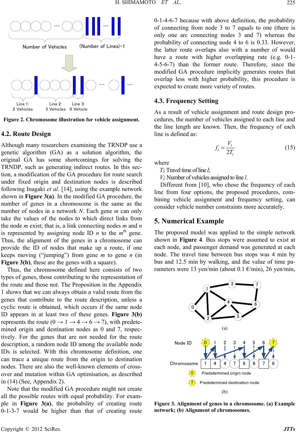 H. SHIMAMOTO ET AL. 225 … … Number of Vehicles(Number of Lines)-1 … … Line 1: 2 Vehicles Line 2: 3 Vehicles Line 3: 0 Vehicle Figure 2. Chromosome illustration for vehicle assignment. 4.2. Route Design Although m g me shortcomings for solving the erating indirect routes. In this sec- from the ge an that of creating route 0- o each line and Then, the frequency of each any researchers examining the TRNDP use a enetic algorithm (GA) as a solution algorithm, the original GA has so TRNDP, such as gen tion, a modification of the GA procedure for route search under fixed origin and destination nodes is described following Inagaki et al. [14], using the example network shown in Figure 3(a). In the modified GA procedure, the number of genes in a chromosome is the same as the number of nodes in a network N. Each gene m can only take the values of the nodes to which direct links from the node m exist; that is, a link connecting nodes m and n is represented by assigning node ID n to the mth gene. Thus, the alignment of the genes in a chromosome can provide the ID of nodes that make up a route, if one keeps moving (“jumping”) from gene m to gene n (in Figure 3(b), these are the genes with a square). Thus, the chromosome defined here consists of two types of genes, those contributing to the representation of the route and those not. The Proposition in the Appendix 1 shows that we can always obtain a valid route nes that contribute to the route description, unless a cyclic route is obtained, which occurs if the same node ID appears in at least two of these genes. Figure 3(b) represents the route (0 → 1 → 4 → 6 → 7), with predete- mined origin and destination nodes as 0 and 7, respec- tively. For the genes that are not needed for the route description, a random node ID among the available node IDs is selected. With this chromosome definition, one can trace a unique route from the origin to destination nodes. There are also the well-known elements of cross- over and mutation within GA optimisation, as described in (14) (See, Appendix 2). Note that the modified GA procedure might not create all the possible routes with equal probability. For exam- ple in Figure 3(a), the probability of creating route 0-1-3-7 would be higher th 1-4-6-7 because with above definition, the probability of connecting from node 3 to 7 equals to one (there is only one arc connecting nodes 3 and 7) whereas the probability of connecting node 4 to 6 is 0.33. However, the latter route overlaps also with a number of would have a route with higher overlapping rate (e.g. 0-1- 4-5-6-7) than the former route. Therefore, since the modified GA procedure implicitly generates routes that overlap less with higher probability, this procedure is expected to create more variety of routes. 4.3. Frequency Setting As a result of vehicle assignment and route design pro- cedures, the number of vehicles assigned t the line length are known. line is defined as: 2 l l l V fT (15) where Tl: Travel time of line l; Vl: Number of vehicles assigned to Different from [10], who chose the frequency of each four options, the proposed procedures, com- bient and frequency setting, can core accurately. at and was generated at each n bus stops was 4 min by line l. line from ning vehicle assignm nsider vehicle number constraints mo 5. Numerical Example The proposed model was applied to the simple network shown in Figure 4. Bus stops were assumed to exist each node, and passenger dem node. The travel time betwee bus and 12.5 min by walking, and the value of time pa- rameters were 13 yen/min (about 0.1 €/min), 26 yen/min, 0 1 3 4 7 6 5 2 (a) 4 7661 467 01234567 Node ID Chromosome 0 7 Pr e de ter m i ned origin n ode Predet e r mined dest inat ion node (b) Figure 3. Alignment of genes in a chromosome. (a) Example network; (b) Alignment of chromosomes. Copyright © 2012 SciRes. JTTs 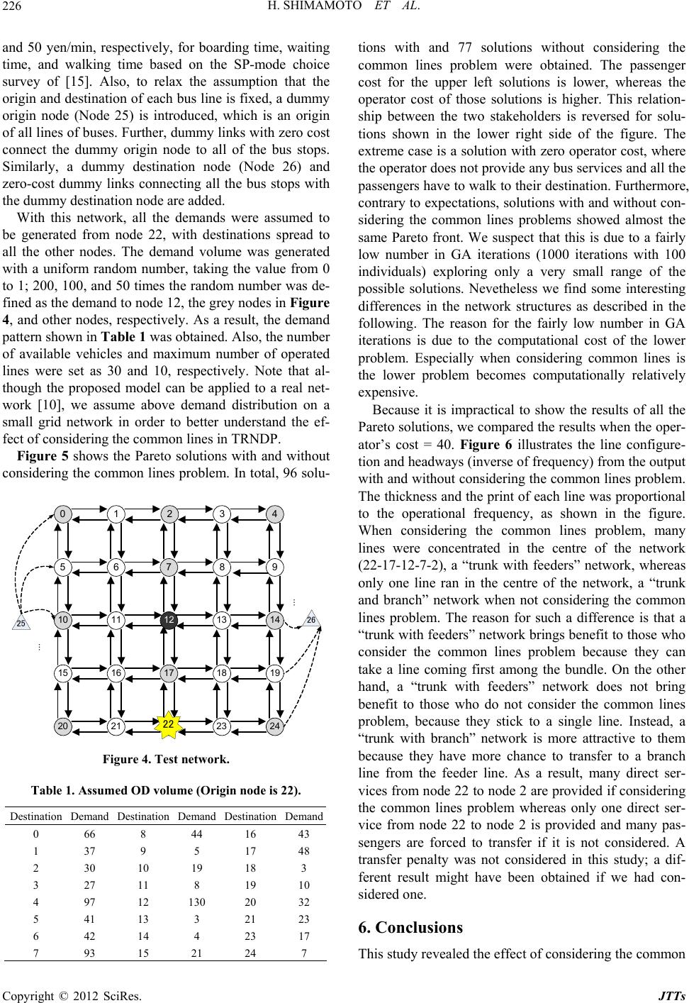 H. SHIMAMOTO ET AL. 226 and 50 yen/min, respectively, for boarding time, waiting time, and walking time based on the SP-mode choice survey of [15]. Also, to rhe origin and destination of eaus line is fixed, a dummy ks with zero cost nodes in Figure 4, tions with and 77 solutions without considering the commn lineroblemere obtained. sser cost he ur leftlution lowehereahe operator cost hose tions higheris reln- ship tween two eholde is revfor- tionsown ihe lowght of figure.he ss and the print of each line was proportional to elax the assum ch b ption that t origin node (Node 25) is introduced, which is an origin of all lines of buses. Further, dummy lin connect the dummy origin node to all of the bus stops. Similarly, a dummy destination node (Node 26) and zero-cost dummy links connecting all the bus stops with the dummy destination node are added. With this network, all the demands were assumed to be generated from node 22, with destinations spread to all the other nodes. The demand volume was generated with a uniform random number, taking the value from 0 to 1; 200, 100, and 50 times the random number was de- fined as the demand to node 12, the grey and other nodes, respectively. As a result, the demand pattern shown in Table 1 was obtained. Also, the number of available vehicles and maximum number of operated lines were set as 30 and 10, respectively. Note that al- though the proposed model can be applied to a real net- work [10], we assume above demand distribution on a small grid network in order to better understand the ef- fect of considering the common lines in TRNDP. Figure 5 shows the Pareto solutions with and without considering the common lines problem. In total, 96 solu- 12 34 56 78 9 10 1113 14 15 161718 19 20 212223 24 0 12 25 26 … … 22 Figure 4. Test network. Table 1. Assumed OD volume (Ori gin node is 22). Destination Demand Destination Demand DestinationDemand 0 66 8 44 16 43 1 37 48 2 30 10 19 18 3 9 5 17 3 27 11 8 19 10 4 97 12 130 20 32 5 41 13 3 21 23 6 42 14 4 23 17 7 93 15 21 24 7 os p wThe paeng for tppe sos isr, ws t of tsoluis . Thatio bethestakrsersed solu shn ter ri sidethe T extreme case is a solution with zero operator cost, where the operator does not provide any bus services and all the passengers have to walk to their destination. Furthermore, contrary to expectations, solutions with and without con- sidering the common lines problems showed almost the same Pareto front. We suspect that this is due to a fairly low number in GA iterations (1000 iterations with 100 individuals) exploring only a very small range of the possible solutions. Nevetheless we find some interesting differences in the network structures as described in the following. The reason for the fairly low number in GA iterations is due to the computational cost of the lower problem. Especially when considering common lines is the lower problem becomes computationally relatively expensive. Because it is impractical to show the results of all the Pareto solutions, we compared the results when the oper- ator’s cost = 40. Figure 6 illustrates the line configure- tion and headways (inverse of frequency) from the output with and without considering the common lines problem. The thickne the operational frequency, as shown in the figure. When considering the common lines problem, many lines were concentrated in the centre of the network (22-17-12-7-2), a “trunk with feeders” network, whereas only one line ran in the centre of the network, a “trunk and branch” network when not considering the common lines problem. The reason for such a difference is that a “trunk with feeders” network brings benefit to those who consider the common lines problem because they can take a line coming first among the bundle. On the other hand, a “trunk with feeders” network does not bring benefit to those who do not consider the common lines problem, because they stick to a single line. Instead, a “trunk with branch” network is more attractive to them because they have more chance to transfer to a branch line from the feeder line. As a result, many direct ser- vices from node 22 to node 2 are provided if considering the common lines problem whereas only one direct ser- vice from node 22 to node 2 is provided and many pas- sengers are forced to transfer if it is not considered. A transfer penalty was not considered in this study; a dif- ferent result might have been obtained if we had con- sidered one. 6. Conclusions This study revealed the effect of considering the common Copyright © 2012 SciRes. JTTs 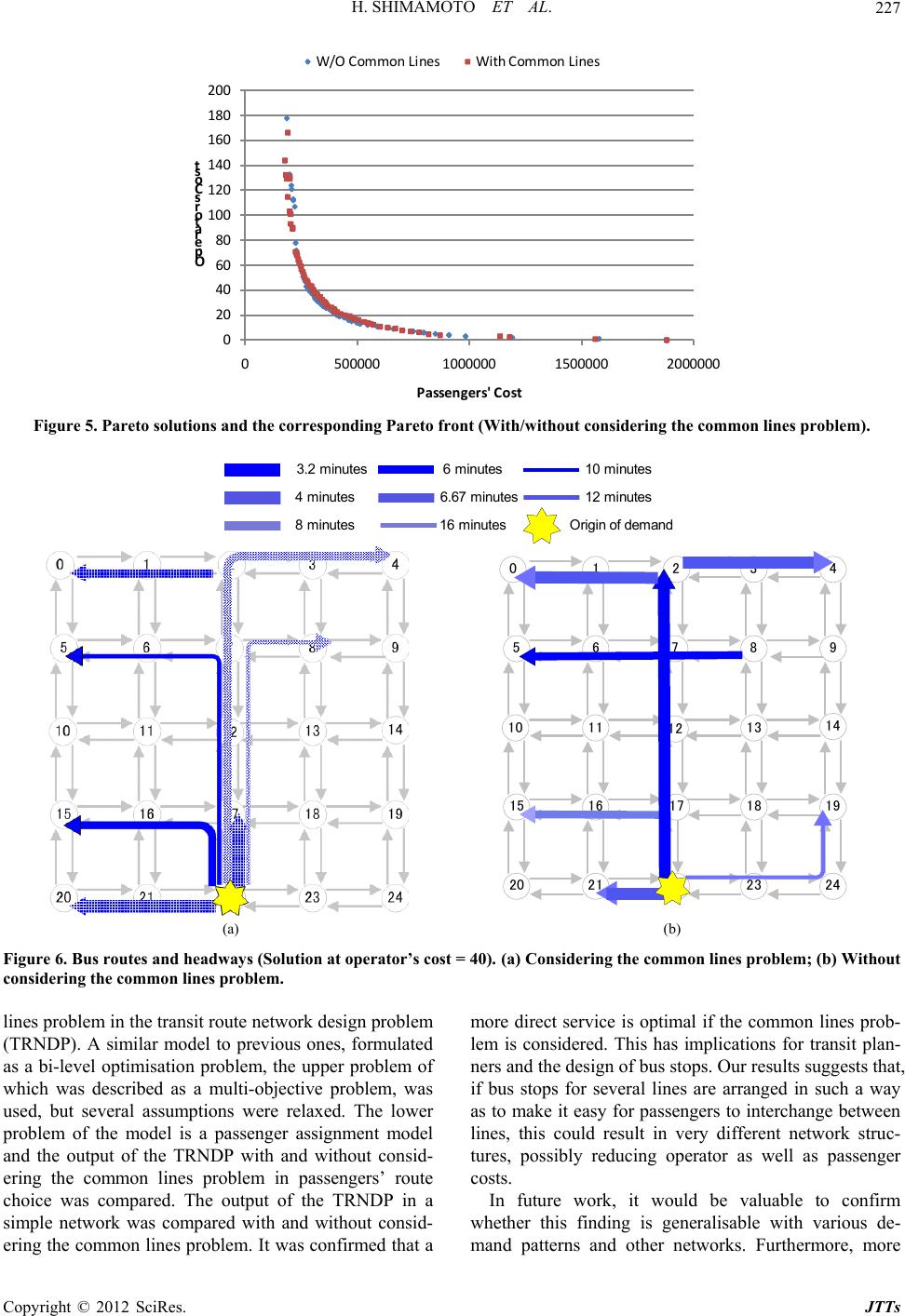 H. SHIMAMOTO ET AL. Copyright © 2012 SciRes. JTTs 227 0 20 40 60 80 100 120 140 160 180 200 05000001000000 1500000 2000000 O p e r a t o r ' s C o s t Passengers' Cost W/O Common LinesWith Common Lines Figure 5. Pareto solutions and the corresponding Pareto front (With/without considering the common lines problem). 3.2 m i nutes6 m in utes10 m inutes 4 m inut es6. 67 m inut es12 m inutes 8 m inut es16 minut esOrigin of demand 4 58 9 11 13 15 18 19 20 012 3 6 7 14 10 12 16 17 21 22 23 24 (a) (b) Figure 6. Bus routes and headways (Solution at operator’s cost = 40). (a) Considering the common lines problem; (b) Without considering the common lines problem. s ones, formulated s a bi-level optimisation problem, the upper problem of lem is considered. This has implications for transit plan- ners and the design of bus stops. Our results suggests that, lines problem in the transit route network design problem (TRNDP). A similar model to previou more direct service is optimal if the common lines prob- a which was described as a multi-objective problem, was used, but several assumptions were relaxed. The lower problem of the model is a passenger assignment model and the output of the TRNDP with and without consid- ering the common lines problem in passengers’ route choice was compared. The output of the TRNDP in a simple network was compared with and without consid- ering the common lines problem. It was confirmed that a if bus stops for several lines are arranged in such a way as to make it easy for passengers to interchange between lines, this could result in very different network struc- tures, possibly reducing operator as well as passenger costs. In future work, it would be valuable to confirm whether this finding is generalisable with various de- mand patterns and other networks. Furthermore, more 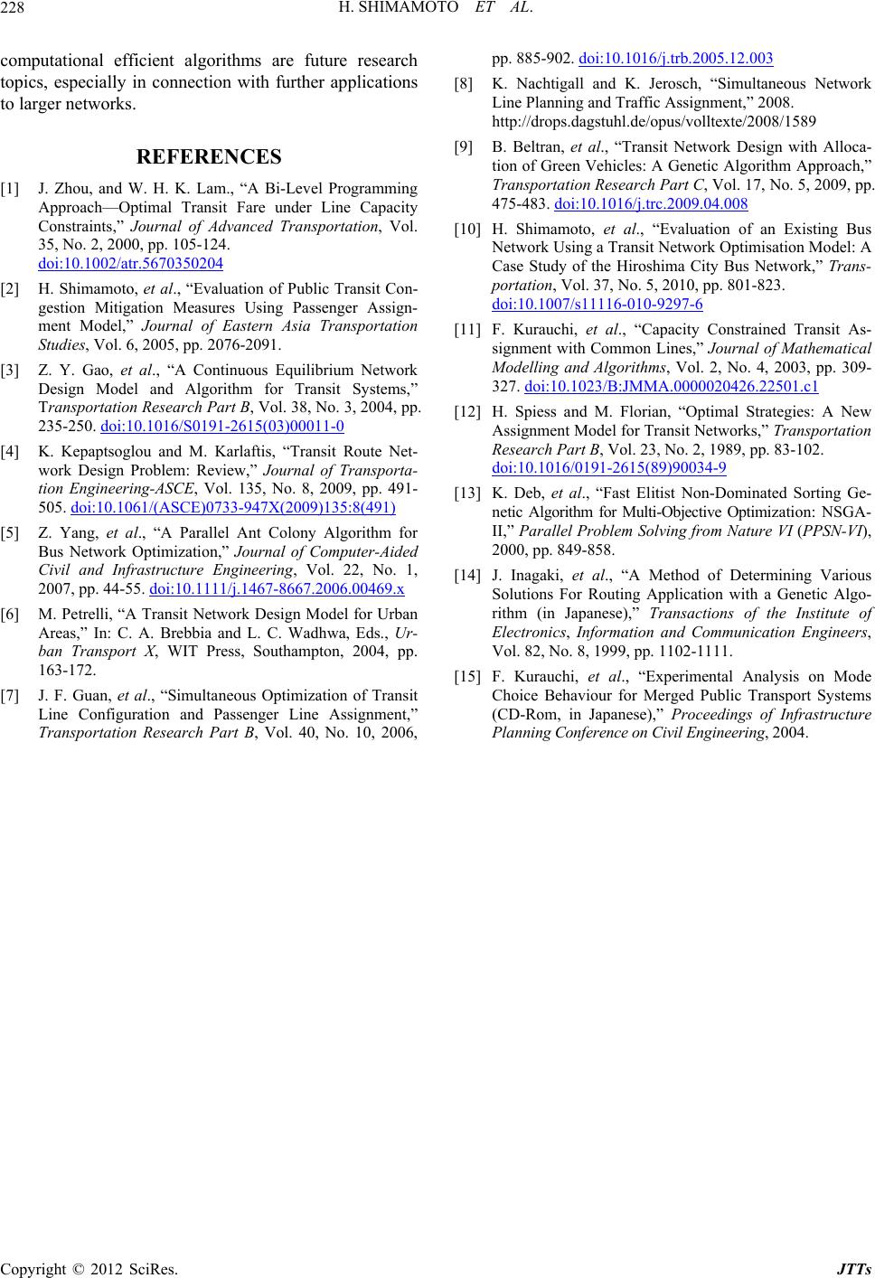 H. SHIMAMOTO ET AL. 228 computational efficient algorithms are future research topics, especially in connection with further applications to larger networks. pp. 105-124. doi:10.1002/atr.5670350204 REFERENCES [1] J. Zhou, and W. H. K. Lam., “A Bi-Level Programming Approach—Optimal Transit Fare under Line Capacity Constraints,” Journal of Advanced Transportation, Vol. 35, No. 2, 2000, [2] H. Shimamotoublic Transit Con- for Transit Syste , et al., “Evaluation of P gestion Mitigation Measures Using Passenger Assign- ment Model,” Journal of Eastern Asia Transportation Studies, Vol. 6, 2005, pp. 2076-2091. [3] Z. Y. Gao, et al., “A Continuous Equilibrium Network Design Model and Algorithmms,” Transportation Research Part B, Vol. 38, No. 3, 2004, pp. 235-250. doi:10.1016/S0191-2615(03)00011-0 [4] K. Kepaptsoglou and M. Karlaftis, “Transit Route Net- work Design Problem: Review,” Journal of Transporta- tion Engineering-ASCE, Vol. 135, No. 8, 2009, pp. 491- 505. doi:10.1061/(ASCE)0733-947X(2009)135:8(491) [5] Z. Yang, et al., “A Parallel Ant Colony Algorithm for Bus Network Optimization,” Journal of Computer-Aided Civil and Infrastructure Engineering, Vol. 22, No. 1, 2007, pp. 44-55. doi:10.1111/j.1467-8667.2006.00469.x [6] M. Petrelli, “A Transit Network Design Model for Urban Areas,” In: C. A. Brebbia and L. C. Wadhwa, Eds., Ur- ban Transport X, WIT Press, Southampton, 2004, pp. 163-172. [7] J. F. Guan, et al., “Simultaneous Optimization of Transit Line Configuration and Passenger Line Assignment,” Transportation Research Part B, Vol. 40, No. 10, 2006, pp. 885-902. doi:10.1016/j.trb.2005.12.003 [8] K. Nachtigall and K. Jerosch, “Simultaneous Network Line Planning and Traffic Assignment,” 2008. http://drops.dagstuhl.de/opus/volltexte/2008/1589 roach,” 09, pp. [9] B. Beltran, et al., “Transit Network Design with Alloca- tion of Green Vehicles: A Genetic Algorithm App Transportation Research Part C, Vol. 17, No. 5, 20 475-483. doi:10.1016/j.trc.2009.04.008 [10] H. Shimamoto, et al., “Evaluation of an Existing Bus Network Using a Transit Network Optimisation Model: A Case Study of the Hiroshima City Bus Network,” Trans- portation, Vol. 37, No. 5, 2010, pp. 801-823. doi:10.1007/s11116-010-9297-6 [11] F. Kurauchi, et al., “Capacity Constrained Transit As- signment with Common Lines,” Journal of Ma Modelling and Algorithms, Vol. thematical 2, No. 4, 2003, pp. 309- 327. doi:10.1023/B:JMMA.0000020426.22501.c1 [12] H. Spiess and M. Florian, “Optimal Strategies: A New Assignment Model for Transit Networks,” Transportation Research Part B, Vol. 23, No. 2, 1989, pp. 83-102. doi:10.1016/0191-2615(89)90034-9 [13] K. Deb, et al., “Fast Elitist Non-Dominated Sorting Ge- netic Algorithm for Multi-Objective Optimization: NS II,” Parallel Problem Solving from N GA- ature VI (PPSN-VI), ,” Transactions of the Institute of s of Infrastructure 2000, pp. 849-858. [14] J. Inagaki, et al., “A Method of Determining Various Solutions For Routing Application with a Genetic Algo- rithm (in Japanese) Electronics, Information and Communication Engineers, Vol. 82, No. 8, 1999, pp. 1102-1111. [15] F. Kurauchi, et al., “Experimental Analysis on Mode Choice Behaviour for Merged Public Transport Systems (CD-Rom, in Japanese),” Proceeding Planning Conference on Civil Engineering, 2004. Copyright © 2012 SciRes. JTTs 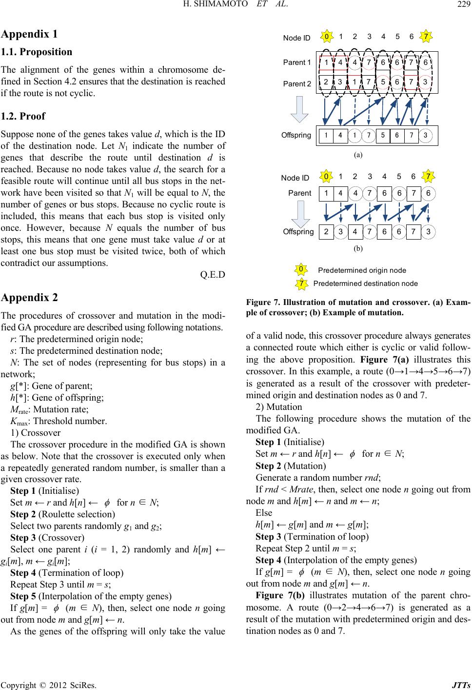 H. SHIMAMOTO ET AL. 229 Appendix 1 osition of the genes within a chromosome de- .2 ensures that the destination is reached clic. s takes value d, which is the ID of the destination node. Let N1 indicate the number of describe the route until destination d is The procedures of crossover and mutation in the fied GA procedure are described using following notations. rmined origin node; er. in the modified GA is shown assover is executed only when a m number, is smaller than a gi 1.1. Prop The alignment fined in Section 4 if the route is not cy 1.2. Proof Suppose none of the gene genes that reached. Because no node takes value d, the search for a feasible route will continue until all bus stops in the net- work have been visited so that N1 will be equal to N, the number of genes or bus stops. Because no cyclic route is included, this means that each bus stop is visited only once. However, because N equals the number of bus stops, this means that one gene must take value d or at least one bus stop must be visited twice, both of which contradict our assumptions. Q.E.D Appendix 2 modi- r: The predete s: The predetermined destination node; N: The set of nodes (representing for bus stops) in a network; g[*]: Gene of parent; h[*]: Gene of offspring; Mrate: Mutation rate; Kmax: Threshold numb 1) Crossover e crure Thossover proced elo bw. Note that the cros erated randorepeatedly gen ven crossover rate. Step 1 (Initialise) Set m ← r and h[n] ← for n ∈ N; Step 2 (Roulette selection) rSelect two parentsandomly g1 and g2; ly and h[m] ← gi Step 3 (Crossover) 2) randomSelect one parent i (i = 1, [m], m ← gi[m]; of loop) Step 4 (Termination Repeat Step 3 until m = s; Step 5 (Interpolation of the empty genes) If g[m] = (m ∈ N), then, n. select one node n going ou ke the value t from node m and g[m] ← As the genes of the offspring will only ta 4 7661 467 01234567 632 371 75 1 731 4576 Paren t 1 Offspr ing Node ID Paren t 2 (a) 4 766146 7 3 732 46 76 Parent Offsprin g 01234567 Nod e ID (b) 0Predete rmined origin node 7Pr edeterm ined destination no de Figure 7. Illustration of mutation and crossover. (a) Exam- ple of crossover; (b) Exampl of a valid node, this crossover procedure alwas generates a connected route which either is cyclic or follow- Figure 7(a) with predeter- e of mutation. y valid ing the above proposition. illustrates this crossover. In this example, a route (0→1→4→5→6→7) s generated as a result of the crossoveri mined origin and destination nodes as 0 and 7. 2) Mutation The following procedure shows the mutation of the modified GA. Step 1 (Initialise) Set m ← r and h[n] ← for n ∈ N; tion) Step 2 (Muta Generate a random number rnd; If rnd < Mrate, then, select one node n going out from node m and h[m] ← n and m ← n; g[ Else ← m]; h[m] ← g[m] and m Step 3 (Termination of loop) Repeat Step 2 until m = s; Step 4 (Interpolation of the empty genes) ] = If g[m (m ∈ N), then, select one node n going ou ion of the parent chro- m→7) is generated as a rend des- tin t from node m and g[m] ← n. Figure 7(b) illustrates mutat →6osome. A route (0→2→4 sult of the mutation with predetermined origin a s andation nodes 0 a 7. Copyright © 2012 SciRes. JTTs
|