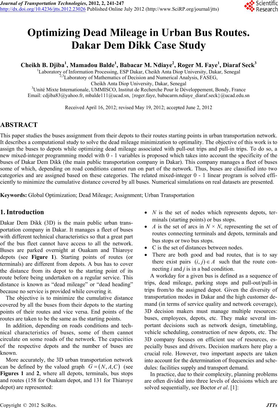
Journal of Transportation Technologies, 2012, 2, 241-247
http://dx.doi.org/10.4236/jtts.2012.23026 Published Online July 2012 (http://www.SciRP.org/journal/jtts)
Optimizing Dead Mileage in Urban Bus Routes.
Dakar Dem Dikk Case Study
Cheikh B. Djiba1, Mamadou Balde1, Babacar M. Ndiaye2, Roger M. Faye1, Diaraf Seck3
1Laboratory of Information Processing, ESP Dakar, Cheikh Anta Diop University, Dakar, Senegal
2,3Laboratory of Mathematics of Decision and Numerical Analysis, FASEG,
Cheikh Anta Diop University, Dakar, Senegal
3Unité Mixte Internationale, UMMISCO, Institut de Recherche Pour le Développement, Bondy, France
Received April 16, 2012; revised May 19, 2012; accepted June 2, 2012
ABSTRACT
This paper studies the buses assignment from their depots to their rou tes startin g po in ts in urb an transpor tation network.
It describes a computation al stu dy to so lve the d ead mileage minimizatio n to op timality. Th e objectiv e of this wo rk is to
assign the buses to depots while optimizing dead mileage associated with pull-out trips and pull-in trips. To do so, a
new mixed-integer programming model with 0 - 1 variables is proposed which takes into account the specificity of the
buses of Dakar Dem Dikk (the main public transportation company in Dakar). This company manages a fleet of buses
some of which, depending on road conditions cannot run on part of the network. Thus, buses are classified into two
categories and are assigned based on these categories. The related mixed-integer 0 - 1 linear program is solved effi-
ciently to minimize the cumulative distance covered by all buses. Numerical simulations on real datasets are presented.
Keywords: Global Optimization; Dead Mileage; Assignment; Urban Transportation
1. Introduction
Dakar Dem Dikk (3D) is the main public urban trans-
portation company in Dakar. It manages a fleet of buses
with different technical characteristics so that a great part
of the bus fleet cannot have access to all the network.
Buses are parked overnight at Ouakam and Thiaroye
depots (see Figure 1). Starting points of routes (or
terminals) are different from depots. A bus has to cover
the distance from its depot to the starting point of its
route before being undertaken on a regular service. This
distance is known as “dead mileage” or “dead heading”
because no service is provided while covering it.
The objective is to minimize the cumulative distance
covered by all the buses from their depots to the starting
points of their routes and vice versa. End points of the
routes are taken to be the same as the starting points.
In addition, depending on roads conditions and tech-
nical characteristics of buses, some of them cannot
circulate on some roads of the network. The capacities
of the respective depots and the number of buses are
known.
More accurately, the 3D urban transportation network
can be defined by the valued graph (see
Figures 1 and 2, where all depots, terminals, bus stops
and routes (158 for Ou akam depot, and 131 for Thiaroye
depot) are represented:
 ,,
GNAC 
 N is the set of nodes which represents depots, ter-
minals (starti n g points) or bus stops.
 A is the set of arcs in N × N, representing the set of
routes connecting terminals and depots, terminals and
bus stops or two bus stops.
 C is the set of distances between nodes.
 There are both good and bad routes, that is to say
there exist pairs (, )ij A

such that the route con-
necting i and j is in a bad condition.
A workday for a given bus is defined as a sequence of
trips, dead mileage, parking stops and pull-out/pull-in
trips from/to the assigned depot. Given the diversity of
transportation modes in Dakar and the high cu stomer de-
mand (in terms of service quality and network coverag e),
3D decision makers must manage multiple resources:
buses, employees, depots, etc. They make several im-
portant decisions such as network design, timetabling,
vehicle scheduling, construction of new depots, etc. The
3D company focuses on efficient use of resources, es-
pecially buses and drivers. Decision markers here play a
crucial role. However, two important aspects are taken
into account for the determination of frequencies and sche-
dules: facilities supply and transport demand.
In practice, due to their complexity, planning problems
are often divided into three levels of decisions which are
solved sequentially, see Boctor et al. [1]:
C
opyright © 2012 SciRes. JTTs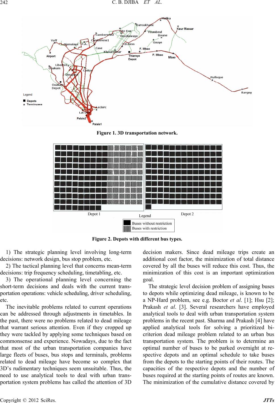

C. B. DJIBA ET AL. 242
Figure 1. 3D transportation network.
Figure 2. Depots with different bus types.
1) The strategic planning level involving long-term
decisions: network design, bus stop problem, etc.
2) The tactical planning level that concerns mean-term
decisions: trip frequency scheduling, timetabling, etc.
3) The operational planning level concerning the
short-term decisions and deals with the current trans-
portation operations: vehicle schedu ling, dr ive r sc hedul ing ,
etc.
The inevitable problems related to current operations
can be addressed through adjustments in timetables. In
the past, there were no problems related to dead mileage
that warrant serious attention. Even if they cropped up
they were tackled by applying some techniques based on
commonsense and experience. Nowadays, due to the fact
that most of the urban transportation companies have
large fleets of buses, bus stops and terminals, problems
related to dead mileage have become so complex that
3D’s rudimentary techniques seem unsuitable. Thus, the
need to use analytical tools to deal with urban trans-
portation system problems has called the attention of 3D
decision makers. Since dead mileage trips create an
additional cost factor, the minimization of total distance
covered by all the buses will reduce this cost. Thus, the
minimization of this cost is an important optimization
goal.
The strategic level decision problem of assigning buses
to depots while optimizing dead mileage, is known to be
a NP-Hard problem, see e.g. Boctor et al. [1]; Hsu [2];
Prakash et al. [3]. Several researchers have employed
analytical tools to deal with urban transportation system
problems in the recent past. Sharma and Prakash [4] have
applied analytical tools for solving a prioritized bi-
criterion dead mileage problem related to an urban bus
transportation system. The problem is to determine an
optimal number of buses to be parked overnight at re-
spective depots and an optimal schedule to take buses
from the depots to the starting points of their routes. Th e
capacities of the respective depots and the number of
buses required at the starting points of routes are known.
The minimization of the cumulative distance covered by

C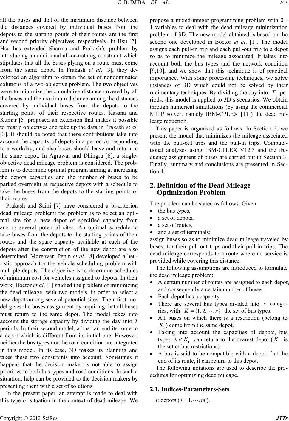. B. DJIBA ET AL. 243
all the buses and that of the maximum distance between
the distances covered by individual buses from the
depots to the starting points of their routes are the first
and second priority objectives, respectively. In Hsu [2],
Hsu has extended Sharma and Prakash’s problem by
introducing an additional all-or-nothing constraint which
stipulates that all the buses plying on a route must come
from the same depot. In Prakash et al. [3], they de-
veloped an algorithm to obtain the set of nondominated
solutions of a two-objectiv e problem. The two objectives
were to minimize the cumulative distance covered by all
the buses and the maximum distance among the distances
covered by individual buses from the depots to the
starting points of their respective routes. Kasana and
Kumar [5] proposed an extension that makes it possible
to treat p objectives and tak e up the data in Prakash et al.
[3]. It should be noted that these contributions take into
account the capacity of depots in a period corresponding
to a workday; and also buses should leave and return to
the same depot. In Agrawal and Dhingra [6], a single-
objective dead mileage problem is considered. The prob-
lem is to determine optimal prog ram aiming at increasing
the depots capacities and the number of buses to be
parked overnight at respective depots with a schedule to
take the buses from the depots to the starting points of
their routes.
Prakash and Saini [7] have considered a bi-criterion
dead mileage problem: the problem is to select an opti-
mal site for a new depot of specified capacity from
among several potential sites. An optimal schedule to
take buses from the depots to the starting points of their
routes and the spare capacity available at each of the
depots after the construction of the new depot are also
determined. Moreover, Pepin et al. [8] developed a heu-
ristic approach for the vehicle scheduling problem with
multiple depots. The objective is to determine schedules
of minimum cost for vehicles assigned to depots. In their
work, Boctor et al. [1] studied the problem of minimizing
the dead mileage, with two models, in order to select a
new depot among several potential sites. Their first mo-
del gives the buses assignment by requiring that all buses
must return to the same depot. The model takes into
account the storage capacity by dividing the day into T
periods. In their second model, a bus can end its route to
a depot which is different from its initial one. However,
neither the bus types no r the road condition are integrated
in this model. In its case, 3D makes its planning and
takes these two constraints into account. Sometimes it
happens that the decision maker is not able to assign
priorities to both bus types and ro ad condition s. In such a
situation, help can be provided to the decision makers by
presenting them with a set of solutio ns.
In the present paper, an attempt is made to deal with
this type of situation in the context of dead mileage. We
propose a mixed-integer programming problem with 0 -
1 variables to deal with the dead mileage minimization
problem of 3D. The new model obtained is based on the
second one developed in Boctor et al. [1]. The model
assigns each pull-in trip and each pull-out trip to a depot
so as to minimize the mileage associated. It takes into
account both the bus types and the network condition
[9,10], and we show that this technique is of practical
importance. With some processing techniques, we solve
instances of 3D which could not be solved by their
rudimentary techniques. By dividing the day into pe-
riods, this model is applied to 3D’s scenarios. We obtain
through numerical simulations (by using the commercial
MILP solver, namely IBM-CPLEX [11]) the dead mi-
leage reduction.
T
This paper is organized as follows: In Section 2, we
present the model that minimizes the mileage associated
with the pull-out trips and the pull-in trips. Computa-
tional analyzes using IBM-CPLEX V12.3 and the fre-
quency assignment of buses are carried out in Section 3.
Finally, summary and conclusions are presented in Sec-
tion 4.
2. Definition of the Dead Mileage
Optimization Problem
The problem can be stated as follows. Given
 the bus types,
 a set of depots,
 a set of routes,
 and a set of terminals;
assign buses so as to minimize dead mileage traveled by
buses, for their pull-out trips and their pull-in trips. The
dead mileage corresponds to a route where no service is
provided while covering th is distance.
The following assumptions are introduced to formulate
the dead mileage problem:
 A certain number of routes are assigned to each depot,
and consequently a certain number of buses.
 Each depot has a capacity.
 There are several bus types divided into r catego-
ries, with

 1,2, ,
Kr

 the set of bus types.
 All buses on which there is a restriction (belong to
1
K
) co me from the same depo t.
 Taking into account the capacities of depots, bus
types 1
kK

can return to the nearest depot (1
K
is
the set of bus restrictions).
 A bus is said to be compatible with a depot if at the
end of its route, it can return to this depot.
The following notations are used to describe the pro-
cedures for optimizing dead mileage.
2.1. Indices-Parameters-Sets
i: depots (1, ,im

).

C. B. DJIBA ET AL. 244
j: routes ().
1,, ,1,,jpp
1, ,tT
n
t: periods ().

k: bus types, . kK
p: number of bus types with restrictions (1 p
K
).
eij: dead mileage associated with the pull-out trip of
route from depot i. j
fij: dead mileage associated with the pull-in trip of
route to depot .
j i
ci: capacity of depot . i
M: total number of available buses for the m depots.
Sit: number of buses leaving fr om depot i at period t.
Rit: number of buses going to depot i at period t.
K: the set of bus types,

 1,2, ,
Kr

.
K1: the set of bus types with restrictions.
2.2. Decision Variables
xij: binary variable which becomes 1 if the pull-out trip
of route j is associated with depot i, 0 otherwise.
yijk: binary variable which becomes 1 if the pull-in trip
of route j is associated with depot i for the bus type k (the
bus which performs the route is compatible to this depot),
0 otherwise.
nit: number of buses in depots i at the beginning of
period t.
The dead mileage problem may be formulated as fol-
lows:
=1 =1=1 =1
min mn mn
ij ijijijk
ij kKij
ex fy


 (1)
s.t.
=1 11,
m
ij
i
,
x
j
n
K
p
K

(2)
=1
11,,
m
ijk
i
yjnk 
 (3)
=1 =1
mn
ijk
kKij
y


 (4)
1
11
it itijijk
jS jR
it it
nnx y



 

(5)
=1, ,2, ,imtTk
1, ,1, ,
it i
nc imtT  (6)
1
=1
m
i
i
nM
 (7)
11 1, , iiT
nni m

 (8)

1, ,1, ,
0,1
ij
x
imjn
kK
,T
(9)
 1, ,1, , 0,1
ijk
yimjn  (10)
01,,1,
it
nimt  (11)
The objective function (1) minimizes the mileage asso-
ciated with the pull-out trips and pull-in trips while tak-
ing into account the bus that covers the route. The de-
parture depots may be different from the return ones. It is
a linear objective function. Constraint (2) implies that the
pull-out trip of a route is associated with a single depot.
Constraint (3) ensures that the pull-in trip is also asso-
ciated with a single depot and takes into account the bus
compatibility. Constraint (4) is effective only when ijk
equals one. It restricts the number of k type bus pull-in
trips to exactly p, where p is the number of bus types
with restrictions. Constraint (5) makes it possible to have,
in real time, the number of buses at each depot. Con-
straint (6) implies that the number of buses in the depot i,
at each period, is less than or equal to the capacity of this
depot. Constraint (7) ensures that the number of buses in
all depots is equal to the number of available buses. Con-
straint (8) ensures the feasibility of the model. The num-
ber of buses in the morning (starting period) must be
equal to the number of buses in the evening (end period).
Constraints (9), (10) and (11) represent domains of the
variables.
y
3. Numerical Experiments
This section shows how the problem is applied to real
data of 3D. Using the model, the operational costs result-
ing from the reduction of dead mileage in urban buses
can be calculated.
Dead mileage does not only have an impact on re-
venue but also in increases of fuel consumption, oper-
ational costs, pollution etc. As all these bad conse-
quences could be reduced with dead mileage, it is thus an
obligation to optimize it.
The operational costs of dead mileage, by a vehicle per
kilometer, is evaluated jointly with 3D. Considering that
the bus average speed is 60 kilometer per hour, the cost
of vehicle use is 1000 FCFA (1.5 euro) per kilo-
meter.

Located at km 4.5 avenue of Cheikh Anta Diop, the
3D company manages a fleet of 410 vehicles using two
depots: a depot located in Ouakam (km 4.5 Cheikh Anta
Diop avenue, the head office of the company) and a de-
pot located in Thiaroye (suburbs of Dakar, 19 kilometers
far from Dakar city).
To ensure network coverage, 3D manages its services
by using 17 lines (see Tables 1 and 2, with 11 from Oua-
kam depot and 6 from Thiaroye depot. Each line ensures
a certain number of routes. Presently, the total number of
routes in the network is 289. Thirty (30) permanent
terminals and 810 bus stops are used (see Figure 1,
where bus stops are not representeddue to their quantity).
The maps in Figures 1 and 3 are obtained by using the
software EMME [12]. A daywork is divided into 38
periods of 30 minutes. The first route of the day should
arrive at its terminal starting at 6:00 am. Given the

C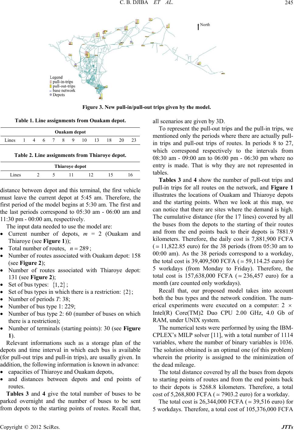. B. DJIBA ET AL. 245
Figure 3. New pull-in/pull-out trips given by the model.
Table 1. Line assignments from Ouakam depot.
Ouakam dep ot
Lines 1 4 6 7 8 910 13 18 2023
Table 2. Line assignments from Thiaroye depot.
Thiaroye depot
Lines 2 5 11 12 15 16
distance between depot and this terminal, the first vehicle
must leave the current depot at 5:45 am. Therefore, the
first period of the model begins at 5:30 am. The first and
the last periods correspond to 05:30 am - 06:00 am and
11:30 pm - 00:00 am, respectively.
The input data needed to use the model are:
 Current number of depots, m = 2 (Ouakam and
Thiaroye (see Figure 1));
 Total number of routes, 289n

;
 Number of routes associated with Ouakam depot: 158
(see Figure 2);
 Number of routes associated with Thiaroye depot:
131 (see Figure 2);
 Set of bus types:
 1,2 ;
 Set of bus types in which there is a restriction: {2};
 Numbe r o f peri o d s T: 38;
 Number of bus type 1: 229;
 Number of bus type 2: 60 (number of buses on which
there is a restriction);
 Number of terminals (starting points): 30 (see Figure
1).
Relevant informations such as a storage plan of the
depots and time interval in which each bus is available
(for pull-out trips and pull-in trips), are usually given. In
addition, the following information is known in advance:
 capacities of Thiaroye and Ouakam depots,
 and distances between depots and end points of
routes.
Tables 3 and 4 give the total number of buses to be
parked overnight and the number of buses to be sent
from depots to the starting points of routes. Recall that,
all scenarios are given by 3D.
To represent the pull-out trips and the pull-in trips, we
mentioned only the periods where there are actually pull-
in trips and pull-out trips of routes. In periods 8 to 27,
which correspond respectively to the intervals from
08:30 am - 09:00 am to 06:00 pm - 06:30 pm where no
entry is made. That is why they are not represented in
tables.
Tables 3 and 4 show the number of pull-out trips and
pull-in trips for all routes on the network, and Figure 1
illustrates the locations of Ouakam and Thiaroye depots
and the starting points. When we look at this map, we
can notice that there are sites where the demand is high.
The cumulative distance (for the 17 lines) covered by all
the buses from the depots to the starting of their routes
and from the end points back to their depots is 7881.9
kilometers. Therefore, the daily cost is 7,881,900 FCFA
(11,822.85 euro) for the 38 periods (from 05:30 am to
00:00 am). As the 38 periods correspond to a workday,
the total cost is 39,409,500 FCFA (59,114.25 euro) for
5 workdays (from Monday to Friday). Therefore, the
total cost is 157,638,000 FCFA (236,457 euro) for a
month (are counted only workdays).


Recall that, our proposed model takes into account
both the bus types and the network condition. The num-
erical experiments were executed on a computer: 2

Intel(R) Core(TM)2 Duo CPU 2.00 GHz, 4.0 Gb of
RAM, under UNIX system.
The numerical tests were performed by using the IBM-
CPLEX’s MILP solver [11], with a total number of 1114
variables, where the number of binary variables is 1036.
The solution obtained is an optimal one (of this problem)
wherein the priority is assigned to the minimization of
the dead mileage.
The total distance covered by all the buses from depots
to starting points of routes and from the end points back
to their depots is 5268.8 kilometers. Therefore, a total
cost of 5,268,800 FCFA (7903.2 euro) for a workday. 
The total cost is 26,344,000 FCFA (39,516 euro) for
5 workdays. Theref ore, a to tal cost of 105,376, 000 FCFA


C. B. DJIBA ET AL. 246
Table 3. Current situation of pull-out trips.
Periods 1 2 3 4 5 6 7Total
Thiaroye pull-out trips 3 25 40 34 19 8 2131
Ouakam pull-out trips 0 20 37 55 35 9 2158
Table 4. Current situation of pull-in trips.
Periods 28 29 30 31 3233 34 35 363738
Thiaroye
pull-in
trips 2 2 11 8 2614 21 26 1371
Ouakam
pull-in
trips 0 5 4 12 3041 40 22 3 10
(158,064 euro) is obtained for a month.
So, with our model we obtain a saving of 52,262,000
FCFA (78,393 euro) monthly, see Table 5 where
distances are in kilometers.

Tables 6 and 7 show the pull-out trips and the pull-in
trips, respectively. First, some modifications in the pull-
out trips are pointed out. With the assignment of 3D we
have 131 and 158 buses assigned to Thiaroye and Oua-
kam depots, respectively. From our numerical experi-
ments we obtain 137 and 152 buses assigned to Thiaroye
and Ouakam depots, respectively. Therefore, 6 routes are
reduced from Ouakam depot and assigned to Thiaroye.
But, the main difference appears in the assignments by
period.
Indeed, for the first period: the 3 Thiaroye pull-out
trips, corresponding to the starting points Parcelles Ass-
ainies, Case and Palais 1 are assigned to Ouakam depot.
During period 2, Ouakam depot loses 2 pull-out trips to
the benefit of Thiaroye depot which has 27. The same
scenario occurs in periods 3 and 4 where, respectively, 4
and 31 additional routes are assigned to Thiaroye depot.
On the other hand, 18, 8 and 2 routes are moved from
Thiaroye depot and assigned to Ouakam depot, for the
periods 5, 6 a nd 7, respectively.
For the pull-in trips, there is no change in the
period. From period 29 to 34, we have respectively 3, 2,
1, 7, 20 and 20 additional routes; assigned to Thia-
roye depot. From period 35 to 38, we obtain respectively
26, 13, 7 and 1 additional routes, assigned to Ouakam
depot.
th
28
Figure 3 illustrates the new pull-in and pull-out trips
at all terminals except depots. At each terminal are repre-
sented the cumulative pull-in and pull-out trips. Trips
from/to depots are ignored in this figure. One can notice
that the amounts of trips are higher in terminals located
in the northern side; the main reason for this fact is that
most of 3D costumers leave suburbs. So during the mor-
ning 3D manages to assign an important quantity of
buses to the suburbs’ terminal to carry people to offices,
factories, firms that are downtown. In the evening the re-
Table 5. Comparison of distances and costs.
Cumulative
distance (km)Current cost (FCFA) Actual distance (km) Actual cost (FCFA) Savings (FCFA)
7881.9 157,638,0005268.8 105,376,00052,262,000
Table 6. New situation of pull-out trips by using the model.
Periods 1 23 4 5 6 7Total
Thiaroye pull-ou t trips02744 65 1 0 0137
Ouakam pull-out trips31833 24 53 17 4152
Table 7. New situation of pull-in trips by using the model.
Periods2829303132 33 34 35 363738
Thiaroye
pull-in
trips 2513933 34 41 0 000
Ouakam
pull-in
trips 0221123 21 20 48 1681
versed phenomenon takes pla ce.
Sites where demand is high correspond to starting
points of Dieupeul, Liberte 6, Palais 1, Guediawaye,
Camberene 1, Daroukhane and Keur Massar. The starting
points of Airport, Camberene 2, Mbao and Malika are the
second category of concentration. The results show that
by allowing buses to return to their starting points or
depots different from the starting ones, we can
significantly reduce the dead mileage, and thus obtain
greater savings. All this database is validated by 3D
officials.
4. Concluding Remarks
In this paper, we described how the new model of opti-
mizing dead mileage can be used to compute an optimal
solution of the 3D urban transportation problem. We
developed a mixed-integer programming problem with 0
- 1 variables which takes into account road network and
achieved greater savings. The results showed that 3D can
significantly reduce the cumulative distance covered by
all the buses from their depots to the starting points of
their routes and also from starting points of their routes
back to their depots. To be more competitive, alterations,
roads repairs, fleet renewal and constructions of new
depots will improve the results performance. Further-
more, the model considered in this work can be used in
the cas e where the en d points of ro utes ar e differ ent from
starting points.
5. Acknowledgements
We would like to thank all DSI’s (Division Système
d’Information) members of 3D for their time and efforts
in providing us with significant improvements of this
paper.

C. B. DJIBA ET AL. 247
REFERENCES
[1] F. F. Boctor, J. Renaud and S. Bournival, “Choix de Sites
D’Entrepôts Pour Les Autobus de Transport Urbain: Le
Cas du Réseau de Transport de La Capitale,” 2006.
http://www.fsa.ulaval.ca/personnel/renaudj/pdf/Recherch
e/RTC%20INFOR.pdf
[2] J. A. Hsu, “Discussion on the Paper: Optimizing Dead
Mileage in Urban Bus Routes,” Journal of Transportation
Engineering, Vol. 114, No. 1, 1988, pp. 123-125.
doi:10.1061/(ASCE)0733-947X(1988)114:1(123)
[3] S. Prakash, B. V. Balaji and D. Tuteja, “Optimizing Dead
Mileage in Urban Bus Routes through a Nondominated
Solution Approach,” European Journal of Operational
Research, Vol. 114, No. 3, 1999, pp. 465-473.
doi:10.1016/S0377-2217(98)00238-0
[4] V. Sharma and S. Prakash, “Optimizing Dead Mileage in
Urban Bus Routes,” Journal of Transportation Engineer-
ing, Vol. 112, No. 1, 1986, pp. 121-129.
doi:10.1061/(ASCE)0733-947X(1986)112:1(121)
[5] H. S. Kasana and K. D. Kumar, “An Efficient Algorithm
for Multiobjective Transportation Problems,” Asia-Paci-
fic Journal of Operational Research, Vol. 17, 2000, pp.
27-40.
[6] A. K. Agrawal and S. L. Dhingra, “An Optimal Program
for Augmentation of Capacities of Depots and Shipment
of Buses from Depots to Starting Points of Routes,” In-
dian Journal of Pure and Applied Mathematics, Vol. 20,
No. 2, 1989, pp. 111-120.
[7] S. Prakash and V. Saini, “Selection of Optimal Site for
New Depot of Specified Capacity with Two Objectives,”
Indian Journal of Pure and Applied Mathematics, Vol. 20,
No. 5, 1989, pp. 425- 432.
[8] A. S. Pepin, G. Desaulniers and A. Hertz, “Comparison of
Heuristic Approaches for the Multiple Depot Vehicle
Scheduling Problem,” Les Cahiers du GERAD, Vol. 65,
2006.
[9] C. B. Djiba, “Optimal Assignment of Routes to a Termi-
nal for an Urban Transport Network. Master of Research
Engineering Sciences,” Cheikh Anta Diop University,
2008.
[10] Full Traffic of Dakar Dem Dikk (2008-2009), Input-
Output File. http://www.demdikk.com
[11] IBM ILOG CPLEX Optimization Studio V12.3, Inc. Us-
ing the CPLEXR Callable Library and CPLEX Barrier
and Mixed Integer Solver Options. 2011.
http://www-01.ibm.com/software/integration/optimizatio
n/cplex-optimization-studio
[12] EMME User’s Manual, 2007.