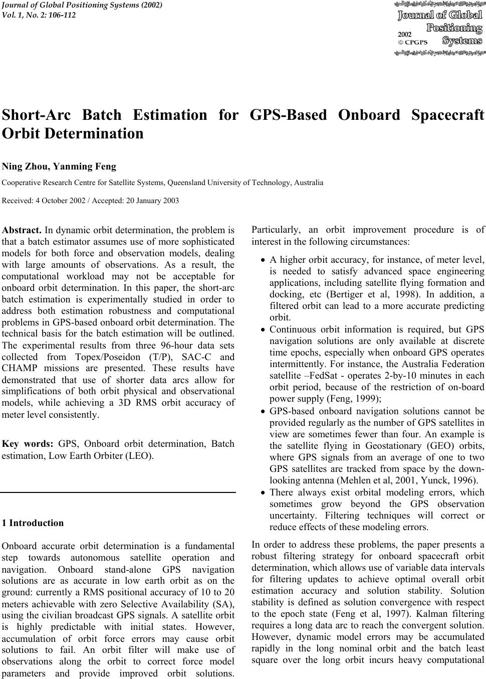
Journal of Global Positioning Systems (2002)
Vol. 1, No. 2: 106-112
Short-Arc Batch Estimation for GPS-Based Onboard Spacecraft
Orbit Determination
Ning Zhou, Yanming Feng
Cooperative Research Centre for Satellite Systems, Queensland University of Technology, Australia
Received: 4 October 2002 / Accepted: 20 January 2003
Abstract. In dynamic orbit determination, the problem is
that a batch estimator assumes use of more sophisticated
models for both force and observation models, dealing
with large amounts of observations. As a result, the
computational workload may not be acceptable for
onboard orbit determination. In this paper, the short-arc
batch estimation is experimentally studied in order to
address both estimation robustness and computational
problems in GPS-based onboard orbit determination. The
technical basis for the batch estimation will be outlined.
The experimental results from three 96-hour data sets
collected from Topex/Poseidon (T/P), SAC-C and
CHAMP missions are presented. These results have
demonstrated that use of shorter data arcs allow for
simplifications of both orbit physical and observational
models, while achieving a 3D RMS orbit accuracy of
meter level consistently.
Key words: GPS, Onboard orbit determination, Batch
estimation, Low Earth Orbiter (LEO).
1 Introduction
Onboard accurate orbit determination is a fundamental
step towards autonomous satellite operation and
navigation. Onboard stand-alone GPS navigation
solutions are as accurate in low earth orbit as on the
ground: currently a RMS positional accuracy of 10 to 20
meters achievable with zero Selective Availability (SA),
using the civilian broadcast GPS signals. A satellite orbit
is highly predictable with initial states. However,
accumulation of orbit force errors may cause orbit
solutions to fail. An orbit filter will make use of
observations along the orbit to correct force model
parameters and provide improved orbit solutions.
Particularly, an orbit improvement procedure is of
interest in the following circumstances:
• A higher orbit accuracy, for instance, of meter level,
is needed to satisfy advanced space engineering
applications, including satellite flying formation and
docking, etc (Bertiger et al, 1998). In addition, a
filtered orbit can lead to a more accurate predicting
orbit.
• Continuous orbit information is required, but GPS
navigation solutions are only available at discrete
time epochs, especially when onboard GPS operates
intermittently. For instance, the Australia Federation
satellite –FedSat - operates 2-by-10 minutes in each
orbit period, because of the restriction of on-board
power supply (Feng, 1999);
• GPS-based onboard navigation solutions cannot be
provided regularly as the number of GPS satellites in
view are sometimes fewer than four. An example is
the satellite flying in Geostationary (GEO) orbits,
where GPS signals from an average of one to two
GPS satellites are tracked from space by the down-
looking antenna (Mehlen et al, 2001, Yunck, 1996).
• There always exist orbital modeling errors, which
sometimes grow beyond the GPS observation
uncertainty. Filtering techniques will correct or
reduce effects of these modeling errors.
In order to address these problems, the paper presents a
robust filtering strategy for onboard spacecraft orbit
determination, which allows use of variable data intervals
for filtering updates to achieve optimal overall orbit
estimation accuracy and solution stability. Solution
stability is defined as solution convergence with respect
to the epoch state (Feng et al, 1997). Kalman filtering
requires a long data arc to reach the convergent solution.
However, dynamic model errors may be accumulated
rapidly in the long nominal orbit and the batch least
square over the long orbit incurs heavy computational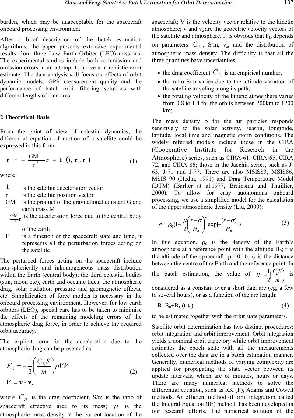

Zhou and Feng: Short-Arc Batch Estimation for Orbit Determination 107
burden, which may be unacceptable for the spacecraft
onboard processing environment.
After a brief description of the batch estimation
algorithms, the paper presents extensive experimental
results from three Low Earth Orbiter (LEO) missions.
The experimental studies include both commission and
omission errors in an attempt to arrive at a realistic error
estimate. The data analysis will focus on effects of orbit
dynamic models, GPS measurement quality and the
performance of batch orbit filtering solutions with
different lengths of data arcs.
2 Theoretical Basis
From the point of view of celestial dynamics, the
differential equation of motion of a satellite could be
expressed in this form:
() rrFrr &&& ,t,
r
GM
3+−=
(1)
where:
r
&& is the satellite acceleration vector
r is the satellite position vector
GM is the product of the gravitational constant G and
earth mass M
r
3
r
GM
− is the acceleration force due to the central body
of the earth
F is a function of the spacecraft state and time, it
represents all the perturbation forces acting on
the satellite
The perturbed forces acting on the spacecraft include
non-spherically and inhomogeneous mass distribution
within the Earth (central body); the third celestial bodies
(sun, moon etc), earth and oceanic tides; the atmospheric
drag, solar radiation pressure and geomagnetic effects,
etc. Simplification of force models is necessary in the
onboard processing environment. However, for low earth
orbiters (LEO), special care has to be taken to minimise
the effects of the remaining modeling errors of the
atmospheric drag force, in order to achieve the required
orbit accuracy.
The explicit term for the acceleration due to the
atmospheric drag can be presented as
a
v-vV
V
=






−= V
m
SC
FD
D
ρ
2
1
(2)
where is the drag coefficient, S/m is the ratio of
spacecraft effective area to its mass; is the
atmospheric mass density at the current location of the
spacecraft; V is the velocity vector relative to the kinetic
atmosphere; v and v
D
C
ρ
a are the geocetric velocity vectors of
the satellite and atmosphere. It is obvious that FD depends
on parameters C, S/m, v
Da, and the distribution of
atmospheric mass density. The difficulty is that all the
three quantities have uncertainties:
0
H
r σ




−
• the drag coefficient is an empirical number,
D
C
• the ratio S/m varies due to the attitude variation of
the satellite traveling along its path;
• the rotating velocity of the kinetic atmosphere varies
from 0.8 to 1.4 for the orbits between 200km to 1200
km;
The mess density ρ for the air particles responds
sensitively to the solar activity, season, longitude,
latitude, local time and magnetic storm conditions. The
widely referred models include those in the CIRA
(Cooperative Institute for Research in the
Atmosphere) series, such as CIRA-61, CIRA-65, CIRA
72, and CIRA 86; those in the Jacchia series, such as J-
65, J-71 and J-77. There are also MSIS83, MSIS86,
MSIS 90 (Hedin, 1991) and Drag Temperature Model
(DTM) (Barlier at al.1977, Bruinsma and Thuillier,
2000). To allow for easy autonomous onboard
processing, we use a simplified model for the calculation
of the upper atmospheric density (Liu, 2000):
])
)(
exp[
2
1(
0
2
0H
r σµ
ρρ
−
−




+= (3)
In this equation, ρ0 is the density of the Earth’s
atmosphere at a reference point with the altitude H0; r is
the altitude of the spacecraft; µ= 0.10, σ is the distance
between the centre of the Earth and the reference point. In
the batch estimation, the value of 





−= m
SC
BD
2
1 is
considered as a constant over a short data arc (eg, a few
to several hours), or as a function of the arc length:
B=B0+B1 (t-t0) (4)
to be estimated together with the orbit state parameters.
Satellite orbit determination has two distinct procedures:
orbit integration and orbit improvement. Orbit integration
yields a nominal orbit trajectory while orbit improvement
estimates the epoch state with all the measurements
collected over the data arc in a batch estimation manner.
Generally, numerical methods of varying complexity are
applied for propagating the state vector between its
update intervals, which are of minutes, hours or days.
There are many numerical methods to solve the
differential equation, such as RK (F), Adams and Cowell
methods. An efficient method of orbit integration, called
the Integral Equation (IE) method, has been developed in
our research efforts. The numerical solution of the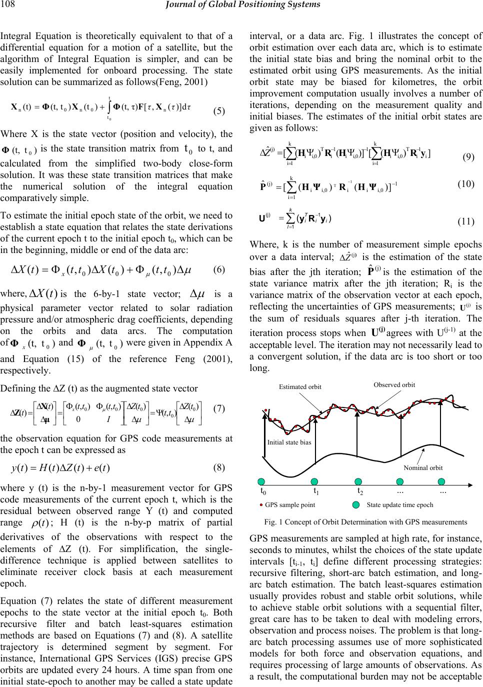

108 Journal of Global Positioning Systems
Integral Equation is theoretically equivalent to that of a
differential equation for a motion of a satellite, but the
algorithm of Integral Equation is simpler, and can be
easily implemented for onboard processing. The state
solution can be summarized as follows(Feng, 2001)
τττ d)](,[τ)(t,)(t)t(t,(t) n
t
t
0n0n
0
XFΦXΦX∫
+=
(5)
Where X is the state vector (position and velocity), the
is the state transition matrix from to t, and
calculated from the simplified two-body close-form
solution. It was these state transition matrices that make
the numerical solution of the integral equation
comparatively simple.
)t(t, 0
Φ0
t
To estimate the initial epoch state of the orbit, we need to
establish a state equation that relates the state derivations
of the current epoch t to the initial epoch t0, which can be
in the beginning, middle or end of the data arc:
µ
µ
∆Φ+∆Φ=∆ ),()(),()( 000 tttXtttX x (6)
where, is the 6-by-1 state vector; is a
physical parameter vector related to solar radiation
pressure and/or atmospheric drag coefficients, depending
on the orbits and data arcs. The computation
of Φand Φwere given in Appendix A
and Equation (15) of the reference Feng (2001),
respectively.
)(tX∆
)t(t,0
µ ∆
x)t(t, 0 µ
Defining the ∆Z (t) as the augmented state vector






∆
∆
Ψ=






∆
∆





ΦΦ
=






∆
∆
=∆
µµ
µ
)(
),(
)(
0
),(),()(
)( 0
0
000 tZ
tt
tZ
I
ttttt
tx
µ
X
Z (7)
the observation equation for GPS code measurements at
the epoch t can be expressed as
)()()()( tetZtHty+∆= (8)
where y (t) is the n-by-1 measurement vector for GPS
code measurements of the current epoch t, which is the
residual between observed range Y (t) and computed
range ; H (t) is the n-by-p matrix of partial
derivatives of the observations with respect to the
elements of ∆Z (t). For simplification, the single-
difference technique is applied between satellites to
eliminate receiver clock basis at each measurement
epoch.
)(t ρ
Equation (7) relates the state of different measurement
epochs to the state vector at the initial epoch t0. Both
recursive filter and batch least-squares estimation
methods are based on Equations (7) and (8). A satellite
trajectory is determined segment by segment. For
instance, International GPS Services (IGS) precise GPS
orbits are updated every 24 hours. A time span from one
initial state-epoch to another may be called a state update
interval, or a data arc. Fig. 1 illustrates the concept of
orbit estimation over each data arc, which is to estimate
the initial state bias and bring the nominal orbit to the
estimated orbit using GPS measurements. As the initial
orbit state may be biased for kilometres, the orbit
improvement computation usually involves a number of
iterations, depending on the measurement quality and
initial biases. The estimates of the initial orbit states are
given as follows:
∑
∑ =
− −
=
− Ψ
Ψ Ψ = ∆ k
1 i i
1
i
T
i,0 i
1
k
1 i i,0
i
1
i
T
i,0 i
(j) ]
) ( [ ] ) ( ) ( [
ˆ y
R H H R H
Z
(9)
1
k
1i
i,0iii,0i
(j) ])()([
ˆ1
T−
=
∑−
=ΨHRΨHP (10)
∑
=
−
=
k
l i
i
T
i
1
1 (j) )
( U y R y
(11)
Where, k is the number of measurement simple epochs
over a data interval; is the estimation of the state
bias after the jth iteration; Pis the estimation of the
state variance matrix after the jth iteration; R
)
(j
ˆ
Z∆
(j)
ˆ
(j)
i is the
variance matrix of the observation vector at each epoch,
reflecting the uncertainties of GPS measurements; U is
the sum of residuals squares after j-th iteration. The
iteration process stops when Uagrees with U
(j)
(j-1) at the
acceptable level. The iteration may not necessarily lead to
a convergent solution, if the data arc is too short or too
long.
t0t1
Observed orbit
Estimated orbit
Nominal orbit
Initial state bias
GPS sample pointState update time epoch
t2··· ···
Fig. 1 Concept of Orbit Determination with GPS measurements
GPS measurements are sampled at high rate, for instance,
seconds to minutes, whilst the choices of the state update
intervals [ti-1, ti] define different processing strategies:
recursive filtering, short-arc batch estimation, and long-
arc batch estimation. The batch least-squares estimation
usually provides robust and stable orbit solutions, while
to achieve stable orbit solutions with a sequential filter,
great care has to be taken to deal with modeling errors,
observation and process noises. The problem is that long-
arc batch processing assumes use of more sophisticated
models for both force and observation equations, and
requires processing of large amounts of observations. As
a result, the computational burden may not be acceptable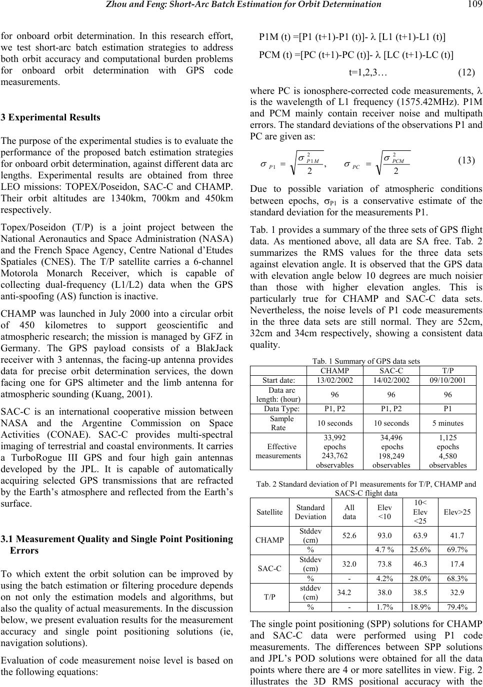

Zhou and Feng: Short-Arc Batch Estimation for Orbit Determination 109
for onboard orbit determination. In this research effort,
we test short-arc batch estimation strategies to address
both orbit accuracy and computational burden problems
for onboard orbit determination with GPS code
measurements.
P1M (t) =[P1 (t+1)-P1 (t)]- λ [L1 (t+1)-L1 (t)]
PCM (t) =[PC (t+1)-PC (t)]- λ [LC (t+1)-LC (t)]
t=1,2,3… (12)
where PC is ionosphere-corrected code measurements, λ
is the wavelength of L1 frequency (1575.42MHz). P1M
and PCM mainly contain receiver noise and multipath
errors. The standard deviations of the observations P1 and
PC are given as:
3 Experimental Results
The purpose of the experimental studies is to evaluate the
performance of the proposed batch estimation strategies
for onboard orbit determination, against different data arc
lengths. Experimental results are obtained from three
LEO missions: TOPEX/Poseidon, SAC-C and CHAMP.
Their orbit altitudes are 1340km, 700km and 450km
respectively.
2
,
2
2 2
1
1
PCM
PC
MP
P
σ
σ
σ
σ
== (13)
Due to possible variation of atmospheric conditions
between epochs, σP1 is a conservative estimate of the
standard deviation for the measurements P1.
Topex/Poseidon (T/P) is a joint project between the
National Aeronautics and Space Administration (NASA)
and the French Space Agency, Centre National d’Etudes
Spatiales (CNES). The T/P satellite carries a 6-channel
Motorola Monarch Receiver, which is capable of
collecting dual-frequency (L1/L2) data when the GPS
anti-spoofing (AS) function is inactive.
Tab. 1 provides a summary of the three sets of GPS flight
data. As mentioned above, all data are SA free. Tab. 2
summarizes the RMS values for the three data sets
against elevation angle. It is observed that the GPS data
with elevation angle below 10 degrees are much noisier
than those with higher elevation angles. This is
particularly true for CHAMP and SAC-C data sets.
Nevertheless, the noise levels of P1 code measurements
in the three data sets are still normal. They are 52cm,
32cm and 34cm respectively, showing a consistent data
quality.
CHAMP was launched in July 2000 into a circular orbit
of 450 kilometres to support geoscientific and
atmospheric research; the mission is managed by GFZ in
Germany. The GPS payload consists of a BlakJack
receiver with 3 antennas, the facing-up antenna provides
data for precise orbit determination services, the down
facing one for GPS altimeter and the limb antenna for
atmospheric sounding (Kuang, 2001).
Tab. 1 Summary of GPS data sets
CHAMP SAC-C T/P
Start date: 13/02/2002 14/02/2002 09/10/2001
Data arc
length: (hour) 96 96 96
Data Type: P1, P2 P1, P2 P1
Sample
Rate 10 seconds 10 seconds 5 minutes
Effective
measurements
33,992
epochs
243,762
observables
34,496
epochs
198,249
observables
1,125
epochs
4,580
observables
SAC-C is an international cooperative mission between
NASA and the Argentine Commission on Space
Activities (CONAE). SAC-C provides multi-spectral
imaging of terrestrial and coastal environments. It carries
a TurboRogue III GPS and four high gain antennas
developed by the JPL. It is capable of automatically
acquiring selected GPS transmissions that are refracted
by the Earth’s atmosphere and reflected from the Earth’s
surface.
Tab. 2 Standard deviation of P1 measurements for T/P, CHAMP and
SACS-C flight data
Satellite Standard
Deviation
All
data
Elev
<10
10<
Elev
<25
Elev>25
Stddev
(cm) 52.6 93.0 63.9 41.7
CHAMP
% 4.7 % 25.6% 69.7%
Stddev
(cm) 32.0 73.8 46.3 17.4
SAC-C
% - 4.2% 28.0% 68.3%
stddev
(cm) 34.2 38.0 38.5 32.9
T/P
% - 1.7% 18.9% 79.4%
3.1 Measurement Quality and Single Point Positioning
Errors
To which extent the orbit solution can be improved by
using the batch estimation or filtering procedure depends
on not only the estimation models and algorithms, but
also the quality of actual measurements. In the discussion
below, we present evaluation results for the measurement
accuracy and single point positioning solutions (ie,
navigation solutions).
The single point positioning (SPP) solutions for CHAMP
and SAC-C data were performed using P1 code
measurements. The differences between SPP solutions
and JPL’s POD solutions were obtained for all the data
points where there are 4 or more satellites in view. Fig. 2
illustrates the 3D RMS positional accuracy with the
Evaluation of code measurement noise level is based on
the following equations: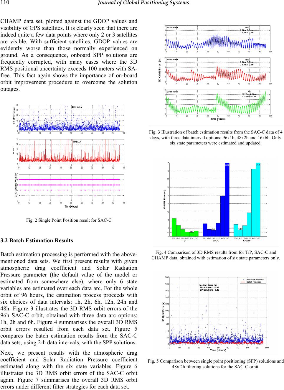

110 Journal of Global Positioning Systems
CHAMP data set, plotted against the GDOP values and
visibility of GPS satellites. It is clearly seen that there are
indeed quite a few data points where only 2 or 3 satellites
are visible. With sufficient satellites, GDOP values are
evidently worse than those normally experienced on
ground. As a consequence, onboard SPP solutions are
frequently corrupted, with many cases where the 3D
RMS positional uncertainty exceeds 100 meters with SA-
free. This fact again shows the importance of on-board
orbit improvement procedure to overcome the solution
outages.
Fig. 3 Illustration of batch estimation results from the SAC-C data of 4
days, with three data interval options: 96x1h, 48x2h and 16x6h. Only
six state parameters were estimated and updated.
Fig. 2 Single Point Position result for SAC-C
3.2 Batch Estimation Results
Fig. 4 Comparison of 3D RMS results from for T/P, SAC-C and
CHAMP data, obtained with estimation of six state parameters only.
Batch estimation processing is performed with the above-
mentioned data sets. We first present results with given
atmospheric drag coefficient and Solar Radiation
Pressure parameter (the default value of the model or
estimated from somewhere else), where only 6 state
variables are estimated over each data arc. For the whole
orbit of 96 hours, the estimation process proceeds with
six choices of data intervals: 1h, 2h, 6h, 12h, 24h and
48h. Figure 3 illustrates the 3D RMS orbit errors of the
96h SAC-C orbit, obtained with three data arc options:
1h, 2h and 6h. Figure 4 summarises the overall 3D RMS
orbit errors resulted from each data set. Figure 5
compares the batch estimation results from the SAC-C
data sets, using 2-h data intervals, with the SPP solutions.
Next, we present results with the atmospheric drag
coefficient and Solar Radiation Pressure coefficient
estimated along with the six state variables. Figure 6
illustrates the 3D RMS orbit errors of the SAC-C orbit
again. Figure 7 summarises the overall 3D RMS orbit
errors under different filter strategies for each data set.
Fig. 5 Comparison between single point positioning (SPP) solutions and
48x 2h filtering solutions for the SAC-C orbit.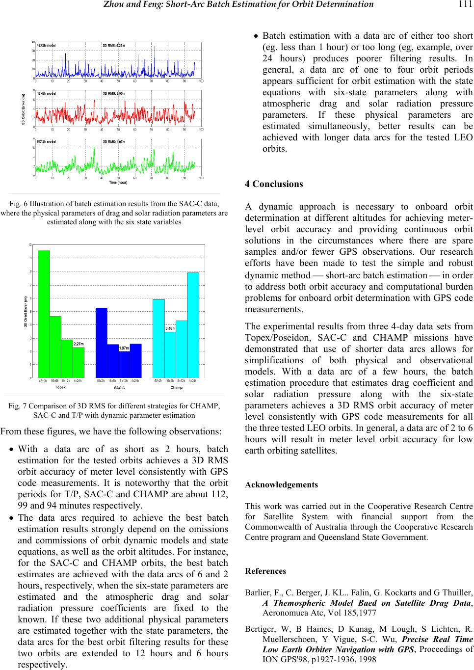

Zhou and Feng: Short-Arc Batch Estimation for Orbit Determination 111
• Batch estimation with a data arc of either too short
(eg. less than 1 hour) or too long (eg, example, over
24 hours) produces poorer filtering results. In
general, a data arc of one to four orbit periods
appears sufficient for orbit estimation with the state
equations with six-state parameters along with
atmospheric drag and solar radiation pressure
parameters. If these physical parameters are
estimated simultaneously, better results can be
achieved with longer data arcs for the tested LEO
orbits.
4 Conclusions
Fig. 6 Illustration of batch estimation results from the SAC-C data,
where the physical parameters of drag and solar radiation parameters are
estimated along with the six state variables
A dynamic approach is necessary to onboard orbit
determination at different altitudes for achieving meter-
level orbit accuracy and providing continuous orbit
solutions in the circumstances where there are spare
samples and/or fewer GPS observations. Our research
efforts have been made to test the simple and robust
dynamic method  short-arc batch estimation  in order
to address both orbit accuracy and computational burden
problems for onboard orbit determination with GPS code
measurements.
The experimental results from three 4-day data sets from
Topex/Poseidon, SAC-C and CHAMP missions have
demonstrated that use of shorter data arcs allows for
simplifications of both physical and observational
models. With a data arc of a few hours, the batch
estimation procedure that estimates drag coefficient and
solar radiation pressure along with the six-state
parameters achieves a 3D RMS orbit accuracy of meter
level consistently with GPS code measurements for all
the three tested LEO orbits. In general, a data arc of 2 to 6
hours will result in meter level orbit accuracy for low
earth orbiting satellites.
Fig. 7 Comparison of 3D RMS for different strategies for CHAMP,
SAC-C and T/P with dynamic parameter estimation
From these figures, we have the following observations:
• With a data arc of as short as 2 hours, batch
estimation for the tested orbits achieves a 3D RMS
orbit accuracy of meter level consistently with GPS
code measurements. It is noteworthy that the orbit
periods for T/P, SAC-C and CHAMP are about 112,
99 and 94 minutes respectively.
Acknowledgements
This work was carried out in the Cooperative Research Centre
for Satellite System with financial support from the
Commonwealth of Australia through the Cooperative Research
Centre program and Queensland State Government.
• The data arcs required to achieve the best batch
estimation results strongly depend on the omissions
and commissions of orbit dynamic models and state
equations, as well as the orbit altitudes. For instance,
for the SAC-C and CHAMP orbits, the best batch
estimates are achieved with the data arcs of 6 and 2
hours, respectively, when the six-state parameters are
estimated and the atmospheric drag and solar
radiation pressure coefficients are fixed to the
known. If these two additional physical parameters
are estimated together with the state parameters, the
data arcs for the best orbit filtering results for these
two orbits are extended to 12 hours and 6 hours
respectively.
References
Barlier, F., C. Berger, J. KL.. Falin, G. Kockarts and G Thuiller,
A Themospheric Model Baed on Satellite Drag Data,
Aeronomuca Atc, Vol 185,1977
Bertiger, W, B Haines, D Kunag, M Lough, S Lichten, R.
Muellerschoen, Y Vigue, S-C. Wu, Precise Real Time
Low Earth Orbiter Navigation with GPS, Proceedings of
ION GPS'98, p1927-1936, 1998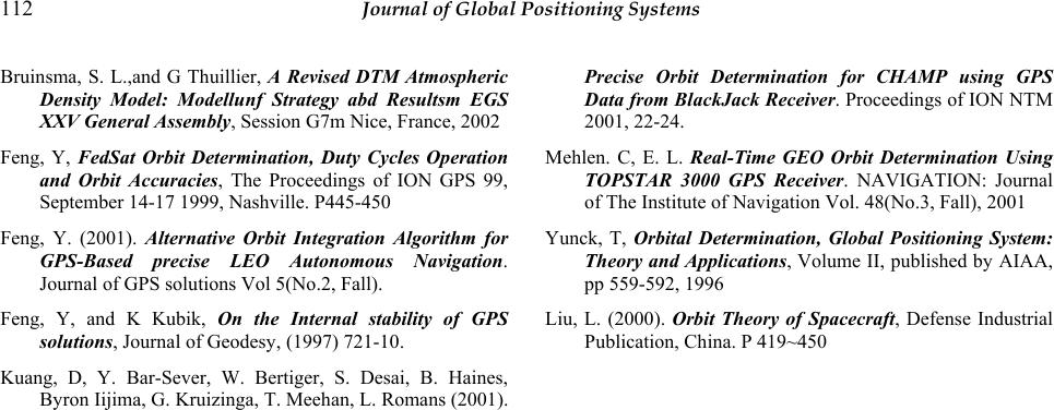

112 Journal of Global Positioning Systems
Bruinsma, S. L.,and G Thuillier, A Revised DTM Atmospheric
Density Model: Modellunf Strategy abd Resultsm EGS
XXV General Assembly, Session G7m Nice, France, 2002
Feng, Y, FedSat Orbit Determination, Duty Cycles Operation
and Orbit Accuracies, The Proceedings of ION GPS 99,
September 14-17 1999, Nashville. P445-450
Feng, Y. (2001). Alternative Orbit Integration Algorithm for
GPS-Based precise LEO Autonomous Navigation.
Journal of GPS solutions Vol 5(No.2, Fall).
Feng, Y, and K Kubik, On the Internal stability of GPS
solutions, Journal of Geodesy, (1997) 721-10.
Kuang, D, Y. Bar-Sever, W. Bertiger, S. Desai, B. Haines,
Byron Iijima, G. Kruizinga, T. Meehan, L. Romans (2001).
Precise Orbit Determination for CHAMP using GPS
Data from BlackJack Receiver. Proceedings of ION NTM
2001, 22-24.
Mehlen. C, E. L. Real-Time GEO Orbit Determination Using
TOPSTAR 3000 GPS Receiver. NAVIGATION: Journal
of The Institute of Navigation Vol. 48(No.3, Fall), 2001
Yunck, T, Orbital Determination, Global Positioning System:
Theory and Applications, Volume II, published by AIAA,
pp 559-592, 1996
Liu, L. (2000). Orbit Theory of Spacecraft, Defense Industrial
Publication, China. P 419~450