Applied Mathematics
Vol.5 No.3(2014), Article ID:42814,19 pages DOI:10.4236/am.2014.53053
Criteria for System of Three Second-Order Ordinary Differential Equations to Be Reduced to a Linear System via Restricted Class of Point Transformation
Department of Mathematics, Faculty of Science, Naresuan University, Phitsanulok, Thailand
Email: supapornsu@nu.ac.th
Received September 11, 2013; revised October 11, 2013; accepted October 18, 2013
ABSTRACT
This paper is devoted to the study of the linearization problem of system of three second-order ordinary differential equations  and
and
 . The necessary conditions for linearization by general point transformation
 and
and  are found. The sufficient conditions for linearization by restricted class of point transformation
 and
and  are obtained. Moreover, the procedure for obtaining the linearizing transformation is provided in explicit forms. Examples demonstrating the procedure of using the linearization theorems are presented.
Keywords:Linearization Problem; Point Transformation; System of Three Second-Order Ordinary Differential Equation
1. Introduction
In general, physical applications of differential equations are in the form of nonlinear equations, which are very difficult to solve explicitly. Most of the solutions are approximate solutions. In solving nonlinear ordinary differential equations, one of the solving methods is reducing nonlinear ordinary differential equations to be linear ordinary differential equations, which makes the method easier and then we have exact solution of original equation.
The first linearization problem for single second-order ordinary differential equations was solved by S. Lie [1]. He found the general form of all ordinary differential equations of second-order that can be reduced to a linear equation by changing the independent and dependent variables. He showed that any linearizable second-order equation should be at most cubic in the first-order derivative and provided a linearization test in terms of its coefficients. The linearization criterion is written through relative invariants of the equivalence group. A. M. Tresse [2] and R. Liouville [3] treated the equivalence problem for second-order ordinary differential equations in terms of relative invariants of the equivalence group of point transformations. In [4] an infinitesimal tech- nique for obtaining relative invariants was applied to the linearization problem. A different approach to tackling the equivalence problem of second-order ordinary differential equations was developed by E. Cartan [5]. The idea of his approach was to associate with every differential equation a uniquely defined geometric structure of a certain form.
The linearization problem for a system of second-order ordinary differential equations was studied in [6,7]. In [6], Wafo and Mahomed found the criteria for linearization of a system of two second-order ordinary differential equations which are related with the existence of an admitted four-dimensional Lie algebra. In [8], Aminova and Aminov gave the necessary and sufficient conditions for a system of second-order ordinary differential equations to be equivalent to the free particle equations. Particular class of systems of two (n = 2) second-order ordinary differential equations was considered by Mahomed and Qadir [9] and they also provided the construction of the linearizing point transformation by using complex variables. Some first-order and second-order relative invariants with respect to point transformations for a system of two ordinary differential equations were obtained in [10]. In [11], Sookmee and Meleshko proposed a new method of linearizing a system of equations, where a given system of equations is reduced to a single equation to which the Lie theorem on linearization is applied. In [12], necessary and sufficient conditions for a system of two second-order ordinary differential equations to be equivalent to the simplest equations were obtained by using the implementation of Cartan’s method. Linearization criteria for a system of two second-order ordinary under general point transformation were obtained in [13]. In [7], linearization criteria for a system of two second-order ordinary differential equations to be equivalent to the linear system with constant coefficients matrix via fiber preserving point transformations were achieved.
Nowadays, the linearization problem of a system of three second-order ordinary differential equations to be equivalent to linear system via point transformations is open. Hence, it’s worth solving this problem as essential part of a study of differential equations.
The manuscript is organized as follows. In Section 2, the necessary conditions of linearization of a system of three second-order ordinary differential equations in the general case of point transformations are presented. In particular, in Section 3, sufficient conditions for linearizing restricted class of point transformations are obtained. Examples which illustrate the procedure of using the linearization theorems are presented in Section 4.
2. Necessary Conditions for Linearization
We begin with investigating the necessary conditions for linearization. We consider a system of three secondorder ordinary differential equations
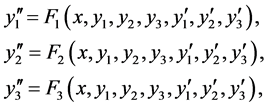 (1)
(1)
which can be transformed to a linear system
 (2)
(2)
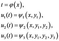
under the point transformation
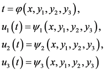 (3)
(3)
So that we arrive at the following theorem.
Theorem 1. Any system of three second-order ordinary differential Equation (1) obtained from a linear system (2) by a point transformation (3) has to be the form
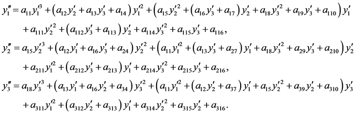 (4)
(4)
where
 (5)
(5)
 (6)
(6)
 (7)
(7)
 (8)
(8)
 (9)
(9)
 (10)
(10)
 (11)
(11)
 (12)
(12)
 (13)
(13)
 (14)
(14)
 (15)
(15)
 (16)
(16)
 (17)
(17)
 (18)
(18)
 (19)
(19)
 (20)
(20)
 (21)
(21)
 (22)
(22)
 (23)
(23)
 (24)
(24)
 (25)
(25)
 (26)
(26)
 (27)
(27)
 (28)
(28)
 (29)
(29)
 (30)
(30)
 (31)
(31)
 (32)
(32)
 (33)
(33)
 (34)
(34)
 (35)
(35)
 (36)
(36)
 (37)
(37)
 (38)
(38)
 (39)
(39)
 (40)
(40)


and

Proof. Applying a point transformation (3), one obtains the following transformation of the first-order derivatives
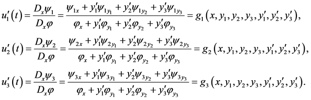
The transformed second-order derivatives are
 (41)
(41)
 (42)
(42)
 (43)
(43)
where


and

is a total derivatives. Replacing 

 into Equations (41)-(43), one gets the system (4). □
3. Sufficient Conditions for Linearization
We have shown in the previous section that every linearizable system of three second-order ordinary differential equations belongs to the class of systems (4). In this section, we formulate the theorem containing sufficient conditions for linearization under the restricted class of point transformation
 (44)
(44)
We arrive at the following theorem.
Theorem 2 System (4) is linearizable by restricted class of point transformation (44) if and only if its coefficients satisfied the following equations
 (45)
(45)
 (46)
(46)
 (47)
(47)
 (48)
(48)
 (49)
(49)
 (50)
(50)
 (51)
(51)
 (52)
(52)
 (53)
(53)
 (54)
(54)
 (55)
(55)
 (56)
(56)
 (57)
(57)
 (58)
(58)
 (59)
(59)
 (60)
(60)
 (61)
(61)
 (62)
(62)
 (63)
(63)
 (64)
(64)
 (65)
(65)
 (66)
(66)
 (67)
(67)
 (68)
(68)
 (69)
(69)
 (70)
(70)
 (71)
(71)
 (72)
(72)
 (73)
(73)
 (74)
(74)
 (75)
(75)
 (76)
(76)
 (77)
(77)
 (78)
(78)
 (79)
(79)
 (80)
(80)
 (81)
(81)
Proof. Since  and
and  are 0, then
  where
where  Considering equation
  one obtains
  From Equations (5)-(7), (9)-(13), (15)-(19), (23), (26) and (28)(29) one gets the conditions

The results from Equations (31)-(34), (8), (21), (22), (25), (27), (38), (36),(37), (14), (20), (24), (37), (39), (30) and (40) can be rewritten as


![]()


![]()

The relation 


 yield the conditions

respectively. Comparing the mixed derivatives

one arrives at the following conditions

respectively. The equations 
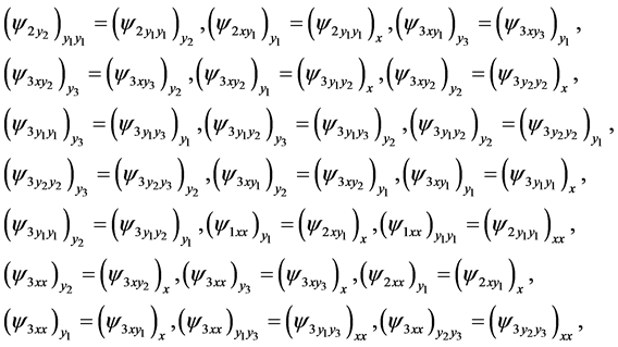
 provide the following conditions:


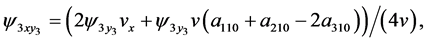
Mixing the derivative  one obtains the derivative

Comparing the mixed derivatives 
 one gets the conditions

All obtained results satisfied the equations 
 □
□
4. Linearizing Transformation
By the prove of Theorem 2, we arrive at the following corollary.
Corollary 3. Provided that the sufficient conditions in Theorem 2 are satisfied, the transformation (44) mapping system (4) to a linear system (2) is obtained by solving the following compatible system of equations for the functions  and
and 
![]() (82)
(82)
 (83)
(83)
 (84)
(84)
 (85)
(85)
 (86)
(86)
 (87)
(87)
 (88)
(88)
 (89)
(89)
 (90)
(90)
 (91)
(91)
 (92)
(92)
 (93)
(93)
 (94)
(94)
 (95)
(95)
 (96)
(96)
 (97)
(97)
 (98)
(98)
 (99)
(99)
 (100)
(100)
 (101)
(101)
 (102)
(102)
5. Examples
Example 1. Consider the system of nonlinear ordinary differential equation.
 (103)
(103)
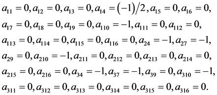
It is a system of the form (4) with the coefficients
 (104)
(104)
One can check that the coefficients (104) obey the conditions (45)-(81). Thus, the Equation (103) is linearizable. We have
 (105)
(105)
 (106)
(106)
 (107)
(107)
 (108)
(108)
 (109)
(109)
 (110)
(110)
 (111)
(111)
 (112)
(112)
 (113)
(113)
 (114)
(114)
 (115)
(115)
 (116)
(116)
 (117)
(117)
 (118)
(118)
 (119)
(119)
 (120)
(120)
 (121)
(121)
 (122)
(122)
 (123)
(123)
 (124)
(124)
 (125)
(125)
From (105) and (106) we get

and

respectively. Since one can use any particular solution, we can take

and this solution satisfies (107). Now the Equation (108) becomes

and yields

Therefore

Since one can use any particular solution, we set and take

Now the Equations (109)-(111) are written
 (126)
(126)
 (127)
(127)
 (128)
(128)
To consider (127) and (128), one takes

then

Since one can use any particular solution, we set  and take

this solution satisfies (126). Now the Equations (112)-(115) are written as
 (129)
(129)
 (130)
(130)
 (131)
(131)
 (132)
(132)
To consider (129), after integration, one finds

Since one can use any particular solution, we set and take

this solution satisfies (130)-(132). Now the Equations (116)-(125) are written
 (133)
(133)
 (134)
(134)
 (135)
(135)
 (136)
(136)
 (137)
(137)
 (138)
(138)
 (139)
(139)
 (140)
(140)
 (141)
(141)
 (142)
(142)
To consider (136), (139), (141) and (142), one obtains

so that

Since one can use any particular solution, we set and take

this solution satisfies (133)-(135), (137)-(138) and (140). Then, one obtains the following transformations
 (143)
(143)
Hence, the system (103) is mapped by the transformations (143) to the linear system

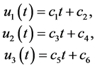
The solution of this linear system is
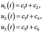
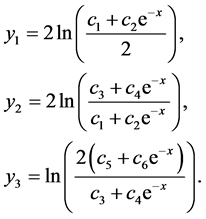
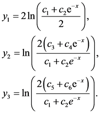
where  are arbitrary constants. By using the transformation (143), one finds

Hence, the solution of the system (103) is
Example 2. Consider the system of nonlinear ordinary differential equation
 (144)
(144)
It is a system of the form (4) with the coefficients
 (145)
(145)
One can check that the coefficients (145) obey the conditions (45)-(81). Thus, the Equation (144) is linearizable. We have
 (146)
(146)
 (147)
(147)
 (148)
(148)
 (149)
(149)
 (150)
(150)
 (151)
(151)
 (152)
(152)
 (153)
(153)
 (154)
(154)
 (155)
(155)
 (156)
(156)
 (157)
(157)
 (158)
(158)
 (159)
(159)
 (160)
(160)
 (161)
(161)
 (162)
(162)
 (163)
(163)
 (164)
(164)
 (165)
(165)
 (166)
(166)
From (146) and (147) we get

and

respectively. Since one can use any particular solution, we can take

and this solution satisfies (148). Now the Equation (149) becomes

and yields

Thus

Since one can use any particular solution, we set and take

Now the Equations (150)-(152) are written
 (167)
(167)
 (168)
(168)
 (169)
(169)
To consider (168) and (169), one gets

Then

Since one can use any particular solution, we set  and take

this solution satisfies (167). Now the Equations (153)-(156) are written as
 (170)
(170)
 (171)
(171)
 (172)
(172)
 (173)
(173)
To consider (170), after integration, one finds

Since one can use any particular solution, we set  and take

this solution satisfies (171)-(173). Now the Equations (157)-(166) are written
 (174)
(174)
 (175)
(175)
 (176)
(176)
 (177)
(177)
 (178)
(178)
 (179)
(179)
 (180)
(180)
 (181)
(181)
 (182)
(182)
 (183)
(183)
To consider (177), (180) and (183), one takes

so that

Since one can use any particular solution, we set and take

this solution satisfies (174)-(176), (178)-(179), (181)-(182). Then, one obtains the following transformations
 (184)
(184)
Hence, the system (144) is mapped by the transformations (184) to the linear system

The solution of this linear system is
where  re arbitrary constants. By using the transformation (184), one finds

Hence, the solution of the system (144) is
Acknowledgements
This research was financially supported by Thailand Research Fund under Grant no. MRG5580053.
REFERENCES
- S. Lie, “Klassifikation und Integration Vongewöhnlichen Differentialgleichungenzwischen x, y die eine Gruppe von Transformation engestatten. III,” Archiv for Matematikog Naturvidenskab, Vol. 8, No. 4, 1883, pp. 371-427.
- A. M. Tresse, “Détermination des Invariants Ponctuels de l’Équationdifférentielleordinaire du Second Ordre
 ,” Preisschriften der Fürstlichen Jablonowski'schen Gesellschaft XXXII, Leipzig, 1896.
 - R. Liouville, “Sur les Invariants de Certaines Equations Differentielles et Surleurs Applications,” Journal de l’École Polytechnique, Vol. 59, 1889, pp. 7-76.
- N. H. Ibragimov, “Invariants of a Remarkable Family of Nonlinear Equations,” Nonlinear Dynamics, Vol. 30, No. 2, 2002, pp. 155-166. http://dx.doi.org/10.1023/A:1020406015011
- E. Cartan, “Sur les Variétés Àconnexion Projective,” Bulletin de la Société Mathématique de France, Vol. 52, 1924, pp. 205-241.
- C. W. Soh and F. M. Mahomed, “Linearization Criteria for a System of Second-Order Ordinary Differential Equations,” International Journal of Non-Linear Mechanics, Vol. 36, No. 36, 2001, pp. 671-677. http://dx.doi.org/10.1016/S0020-7462(00)00032-9
- S. Sookmee and S. V. Meleshko, “Linearization of Two Second-Order Ordinary Differential Equations via Fiber Preserving Point Transformations,” ISRN Mathematical Analysis, Vol. 2001, 2011, Article ID: 452689. http://dx.doi.org/10.5402/2011/452689
- A. V. Aminova and N. A.-M. Aminov, “Projective Geometry of Systems of Second-Order Differential Equations,” Sbornik: Mathematics, Vol. 197, No. 7, 2006, pp. 951-955. http://dx.doi.org/10.1070/SM2006v197n07ABEH003784
- F. M. Mahomed and A. Qadir, “Linearization Criteria for a System of Second-Order Quadratically Semi-Linear Ordinary Differential Equations,” Nonlinear Dynamics, Vol. 48, No. 4, 2007, pp. 417-422. http://dx.doi.org/10.1007/s11071-006-9095-z
- S. Sookmee, “Invariants of the Equivalence Group of a System of Second-Order Ordinary Differential Equations,” M.S. Thesis, 2005.
- S. Sookmee and S. V. Meleshko, “Conditions for Linearization of a Projectable System of Two Second-Order Ordinary Differential Equations,” Journal of Physics A: Mathematical and Theoretical, Vol. 41, No. 402001, 2008, pp. 1-7.
- S. Neut, M. Petitot and R. Dridi, “ÉlieCartan’s Geometrical Vision or How to Avoid Expression Swell,” Journal of Symbolic Computation, Vol. 44, No. 3, 2009, pp. 261-270. http://dx.doi.org/10.1016/j.jsc.2007.04.006
- Y. Y. Bagderina, “Linearization Criteria for a System of Two Second-Order Ordinary Differential Equations,” Journal of Physics A, Vol. 43, No. 46, 2010, Article ID: 465201.