ABSTRACT

This paper develops an integrating algorithm for fully rheonomous affine constraints and gives theoretical analysis of the algorithm for the completely integrable case. First, some preliminaries on the fully rheonomous affine constraints are shown. Next, an integrating algorithm that calculates independent first integrals is derived. In addition, the existence of an inverse function utilized in the algorithm is investigated. Then, an example is shown in order to evaluate the effectiveness of the proposed method. By using the proposed integrating algorithm, we can easily calculate independent first integrals for given constraints, and hence it can be utilized for various research fields.

1. Introduction

Over the last couple of decades, a lot of researches on nonholonomic systems have been done in the research fields of nonlinear control theory and robotics [1-3]. In addition, sub-Riemannian geometry has also been studied in the research fields of differential geometry and control theory [4,5]. The common property in these two is the existence of constraints. The constraints play important roles in these research fields and yield attractive and interesting characteristics.

The simplest class of constraints is linear constraints:, , , and they have been mainly studied so far. The class of the linear constraints covers wide-ranging mechanical systems such as mobile and acrobatic robots. However, there also exist wider classes of constraints. The author has focused and researched scleronomous affine constraints:

, and A-rheonomous affine constraints:, which form a wider class of constraints than the linear constraints, from the viewpoints of mathematics and control theory [6-10]. Note that in analytical mechanics, the terminology “rheonomous” means “time-varying”, and the opposite word of it is “scleronomous”. The affine constraints can be found in mechanical systems such as space robots with initial angular momenta, a ball on a rotating table, a ship on a running river, and so on. These results have made it possible to treat such constraints systematically, however, we are still interested in fully rheonomous affine constraints: 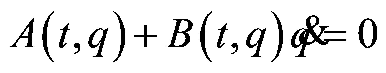as a much wider class of constraints than the $A$-rheonomous affine constraints. In [11], the author has derived a complete integrability condition for the rheonomous affine constraints. If the constraints are integrable, there exist some independent first integrals of them. It is quite important to calculate independent first integrals since they can be utilized for reduction of the configuration space.

Hence, the purpose of this paper is to develop an integrating algorithm for the fully rheonomous affine constraints. This paper is organized as follows. First, in Section 2, some preliminaries on the fully rheonomous affine constraints are presented. Next, in Section 3, an integrating algorithm for completely integrable rheonomous affine constraints is constructed. Moreover, theoretical analysis of the algorithm is shown. Then, Section 4 illustrates an example for verification of the effectiveness and the availability of the new results.

2. Preliminaries

2.1. Fully Rheonomous Affine Constraints

In this section, some preliminaries on fully rheonomous affine constraints are presented. See [11] for more details. First, this subsection gives the definition of fully rheonomous affine constraints and explains their geometric representation. Denote the time variable by and a time interval by. Let be an -dimensional configuration manifold and be a local coordinate of. Associated with, we refer as a tangent vector field. A set of of differenttial equations in the form:

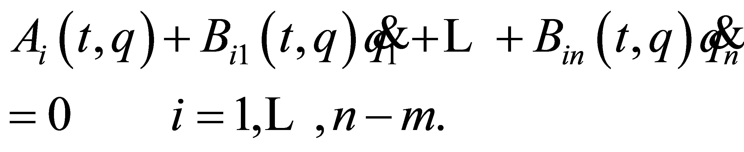(1)

is called fully rheonomous affine constraints. Note that all the coefficients explicitly depend on the time variable. We now rewrite (1) as

(2)

where a rheonomous affine term is a vector-valued function whose -th entry is, and a rheonomous velocity coefficient matrix is a matrix-valued function whose -th entry is. In this paper, we assume the following sufficient condition on independency of the fully rheonomous affine constraints (2):

(3)

Next, a geometric representation method of the fully rheonomous affine constraints (2) is explained. From (1), we see that the row vectors of in (2) are independent of each other. Hence, we consider vector fields which are independent of each other and annihilators of the row vectors of, and denote them by as time-varying vector fields on. Furthermore, we also denote a space spanned by, that is, a time-varying distribution on by

(4)

Since the basial vectors of: are independent of each other, is a nonsingular distribution, that is,

(5)

holds. A curve on: is said to satisfy the fully rheonomous affine constraints (2) if for a timevarying vector field on: and the generalized velocity of:,

(6)

We call a rheonomous affine vector field, and it satisfies the equation:

(7)

This definition is a natural extension of the one for the scleronomous affine constraints that do not contain the time variable explicitly [6]. Geometric representation of the fully rheonomous affine constraints is defined as follows and can allow us to analyze them geometrically and derive geometric properties.

Definition 1

The fully rheonomous affine constraints (2) are geometrically represented by a pair, where is an -dimensional time-varying distribution defined by (4) and is called a rheonomous affine vector and satisfies (7).

2.2. Rheonomous Bracket

Next, in this subsection, a new operator for the fully rheonomous affine constraints (2), called the rheonomous bracket is shown. The rheonomous bracket is originally introduced in order to analyze the A-rheonomous affine constraints in [8-10] and plays important roles in derivation of a complete integrability condition and an integrating algorithm. The rheonomous bracket is fundamentally defined based on the normal Lie bracket, which is an operator for two vector fields:

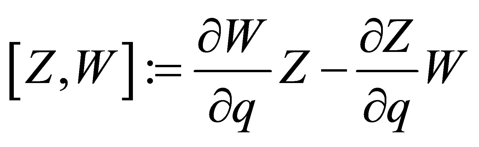(8)

The definition of the rheonomous bracket is as follows. [8-10].

Definition 2 [8-10]

For the vector fields defined on on the geometric representation of the fully rheonomous affine constraints (2):, the rheonomous bracket is an operator: that satisfies the following three properties:

a) For a rheonomous affine vector field,

(9)

Holds.

b) is defined as a set of vector fields that consists of and iterated rheonomous brackets of and does not contain. For a rheonomous affine vector field and a vector field,

(10)

Holds.

c) For two vector fields,

(11)

holds.

For the rheonomous bracket, it is noted that the rheonomous affine vector field is perceived as special, and this yields an additional term of a time differenttial of a vector field as the property (b). It must be also noted that from Definition 2 the rheonomous bracket is equivalent to the normal Lie bracket for scleronomous affine constraints, that is, constraints that do not contain the time variable explicitly. The following proposition shows that the rheonomous bracket has some important characteristics in common with the normal Lie bracket [8-10].

Proposition 1 [8-10]

For the vector fields on the geometric representation of the fully rheonomous affine constraints (2): and the set of iterated vector fields of them:, the following properties (a), (b), and (c) hold.

a) Bilinearlity:

(12)

b) Skew-symmetry:

(13)

c) Jacobi’s identity:

(14)

From the properties in Proposition 1, it can be confirmed that we only have to consider the iterated rheonomous brackets in the form:

(15)

in checking a complete integrability condition for the fully rheonomous affine constraints, which will be shown in the next subsection. Furthermore, the Philip Hall basis [12], which is a systematic method to generate iterated Lie brackets with an order efficiently, can be also constructed for the rheonomous bracket as follows [8-10].

Algorithm 1

For iterated rheonomous brackets (15) of the geometric representation of the fully rheonomous affine constraints (2):, we define the length of (15) as, that is, the number of vector fields in the iterated rheonomous bracket. In addition, the symbol means the magnitude relation for two iterated rheonomous brackets. Then, the Philip Hall basis for the rheonomous bracket can be constructed by the next rules.

a) are the first elements of and.

b) If, then.

c) if and only if and, either or holds or with and.

2.3. Complete Integrability Condition

Finally this subsection presents a complete integrability condition for the fully rheonomous affine constraints (2). If all the rheonomous affine constraints (2) are integrable, that is, there exist independent first integrals of (2), then they are said to be completely integrable. We now define a smallest and involutive timevarying distribution that contains and iterated rheonomous brackets of them, and satisfies that is, is spanned by all the rheonomous brackets of with the exception of. Then, a necessary and sufficient condition on complete integrability for the fully rheonomous affine constraints (2) is given as the next theorem [11].

Theorem 1 [11]

For the fully rheonomous affine constraints defined on an $n$-dimensional manifold (2) and a time interval, the following statements (a) and (b) are equivalent to each other. If they hold, the fully rheonomous affine constraints (2) are said to be completely integrable.

a) There exist independent first integrals of the fully rheonomous affine constraints (2).

b) For a smallest and involutive time-varying distribution,

(16)

holds.

From Theorem 1, we can see that the complete integrability condition for the fully rheonomous affine constraints (2) is quite simple and has a similar structure as the ones for the scleronomous affine constraints and the A-rheonomous affine constraints [6,7]. In addition, it turns out that the rheonomous bracket plays a significant role in the condition (16).

3. Integrating Algorithm

3.1. Proposed Integrating Algorithm

As seen in Section 2, if the fully rheonomous affine constraints (2) are completely integrable, there exist some independent first integrals of them. For reduction of the dimension of a given configuration manifold subject to completely integrable fully rheonomous affine constraints, we need the explicit forms of independent first integrals of them. For scleronomous linear constraints, that is, , a method of calculation of independent first integrals is well known [12,13], and for scleronomous affine constraints: and A-rheonomous affine constraints: we have developed algorithms to calculate independent first integrals of them in [7,9,10]. However, a method to calculate independent first integrals of given fully rheonomous affine constraints has not been proposed. Therefore, this section of the paper develops an integrating algorithm for the fully rheonomous affine constraints and gives theoretical analysis of the algorithm.

In this subsection, we derive an integrating algorithm for completely integrable fully rheonomous affine constraints (2). Theorem 1 in Section 2 guarantees the existence of independent first integrals of the fully rheonomous affine constraints (2). Hence, we aim to construct an algorithm to calculate these $n-m$ independent first integrals. First of all, we can find vector fields such that

(17)

holds for the vector fields of the geometric representtation for the fully rheonomous affine constraints (2):. Let us denote flows (1-parameter local transformation groups) of and by and with time parameters and, respectively. We set an initial point at the initial time as. We also consider vector fields defined on the expanded configuration manifold, and then their flows on are represented as

(18)

Note that the initial value of is set as 0. Calculating the composite mapping of flows (18) yields

(19)

where

(20)

is the composite mapping of flows . From (19), we see that the projection of onto is equivalent to. Therefore, by applying the idea of the integrating algorithm for scleraonomous linear constraints defined on [14,15] to and considering projection of it onto, we can derive the following algorithm to calculate independent first integrals of completely integrable fully rheonomous affine constraints as follows.

Algorithm 2

For the completely integrable fully rheonomous affine constraints (2), we can obtain $n-m$ independent first integrals of them by the following procedure.

(Step 1) Set vector fields of geometric representation for the fully rheonomous affine constraints (2).

(Step 2) For, derive linearly independent vector fields that satisfy (17).

(Step 3) Calculate flows of and set them as.

(Step 4) Combine flows as (20).

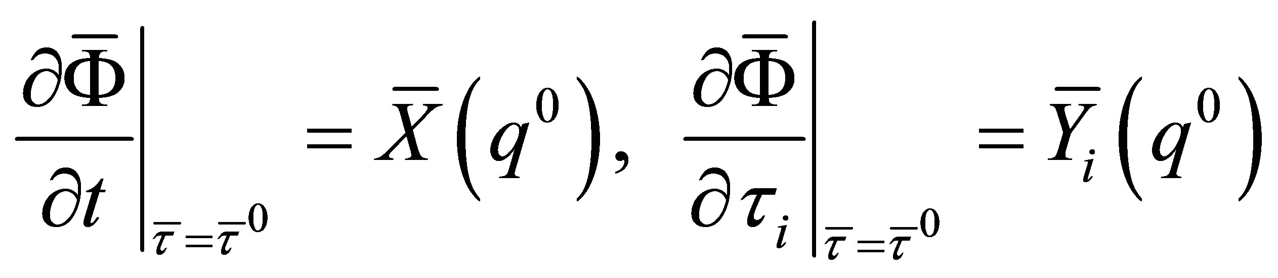
(Step 5) Set and derive the inverse function, where. Then, the last components of are independent first integrals of (2).

It must be noted that Algorithm 1 is similar to the ones for the scleronomous affine constraints case and the Arheonomous affine constraints case [7,9,10], and hence Algorithm 2 is a natural extension of them.

3.2. Theoretical Analysis

This subsection gives theoretical analysis on the integrating algorithm for completely integrable rheonomous affine constraints. In Algorithm 2 derived in the previous subsection, we need to calculate the inverse function of the combined mapping: in order to calculate independent first integrals. However, we still have a important question on the existence of the inverse function. In general, it is quite difficult to calculate an inverse function of a given function. For Algorithm 2, the next proposition guarantees the existence of the inverse mapping.

Proposition 2

Assume that the fully rheonomous affine constraints (2) are completely integrable. Then, there exists an time interval and is a diffeomorphism at any time. That is to say, there exists its inverse mapping.

(Proof) Set. Calculating the partial differential of (19) with the chain rule of differential calculation, we have

(21)

Substituting into (21), we obtain

(22)

that is to say,

(23)

Since are linearly independent of each other,

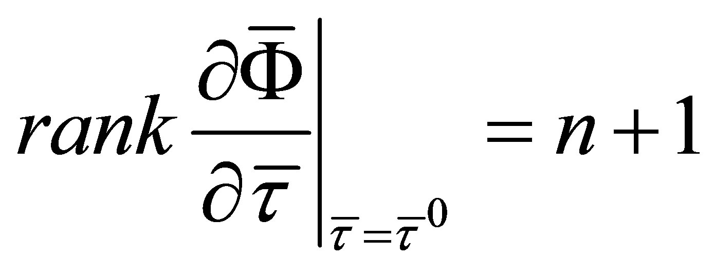(24)

holds. Therefore, it turns out that is a diffeomorphism by the implicit function theorem [12,13]. Since the projection of onto is equivalent to, is also a diffeomorphism. Consequently, the proposition is proven.

4. Example

Finally, in this section, an example is considered in order to evaluate the new results. Let us consider a 3-dimensional configuration manifold:

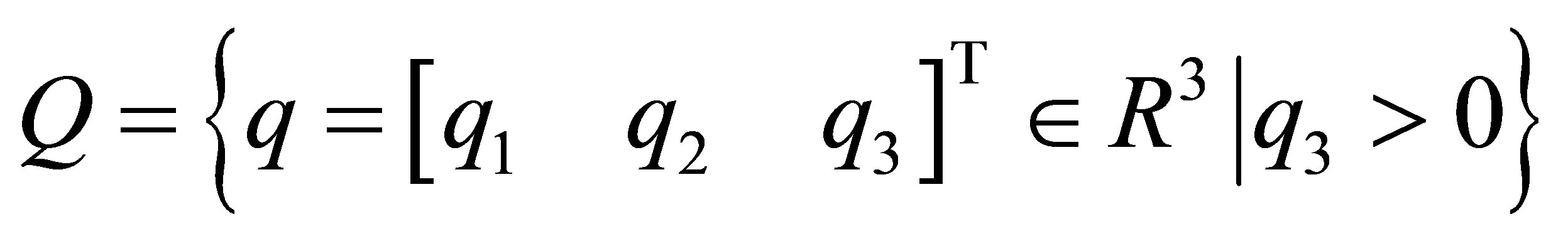(25)

with, and a fully rheonomous affine constraints on:

(26)

with. We here consider a time interval. Then, it turns out that Assumption 1 holds for (26). One geometric representation for (26) can be obtained as follows:

(27)

Calculating an iterated rheonomous bracket for and above, we obtain

(28)

Hence, we can see that all the iterated rheonomous brackets for are 0. Therefore, we have

(29)

and then it can be confirmed that

(30)

holds. From Theorem 1, we can see that the fully rheonomous affine constraints (26) are completely integrable, that is, there exist two independent first integrals of (26).

Next, we shall calculate the first integrals of (26) according to Algorithm 2. Reset and new two vector fields that satisfy (17) as

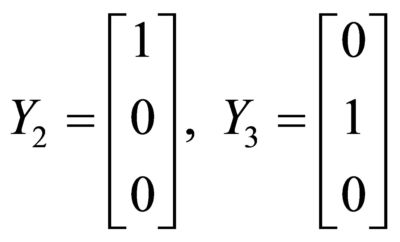(31)

For the vector fields, we calculate their flows as

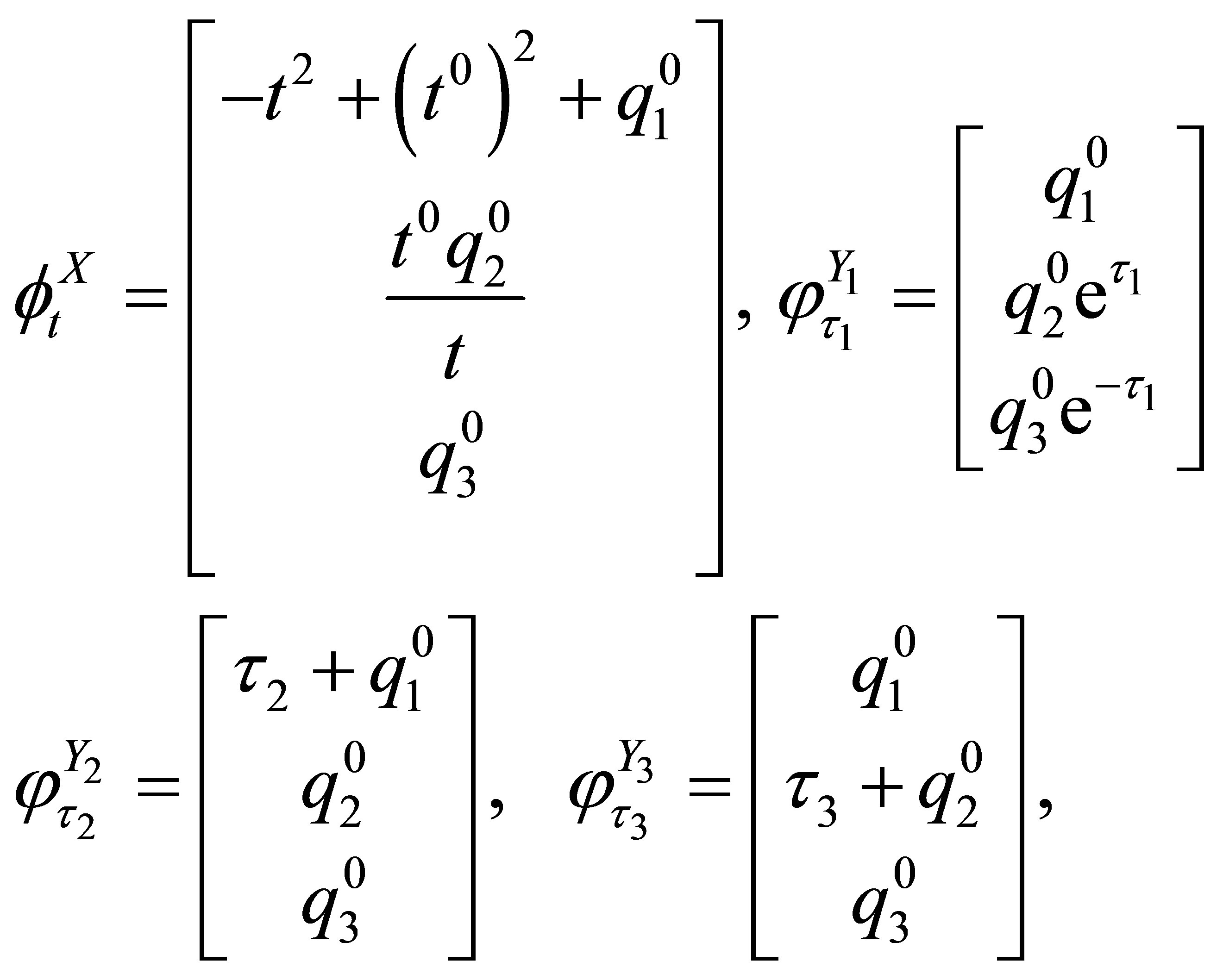(32)

where is the initial point at the initial time. Combining the flows (32) like (20)We have

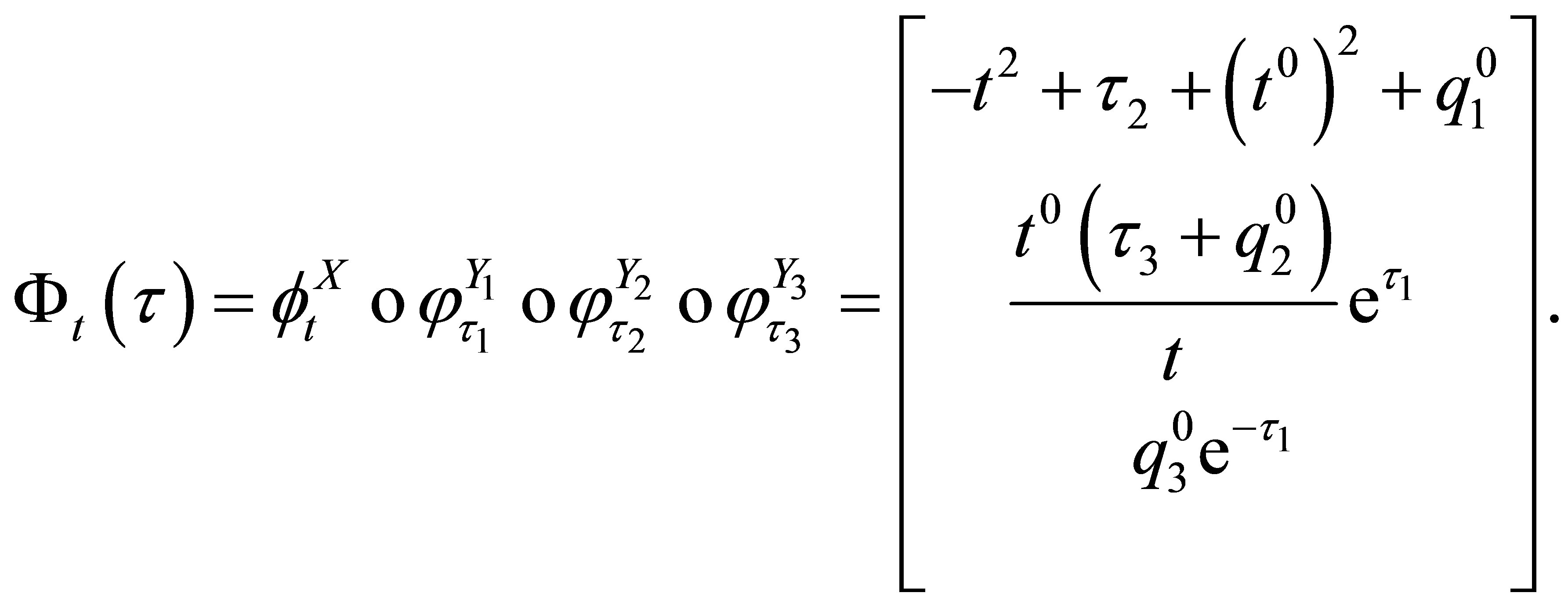(33)

By solving the equation, we calculate the inverse mapping of (33) as

(34)

Consequently, we can obtain two independent first integrals of (26) as the last two components of (34):

(35)

It can be easily checked that the fully rheonomous affine constraints (26) can be derived from two independent first integrals (35).

5. Conclusions

This paper has developed an integrating algorithm in order to calculate independent first integrals for the fully rheonomous affine constraints in the completely integrable case. We can say that the proposed integrating algorithm is useful and has the application potentiality for various research fields.

Future work includes development of integrating algorithm for partially integrable fully rheonomous affine constraints, applications of the algorithm to real systems, and extensions to more general classes of constraints.

REFERENCES

- J. Cortes, “Geometric, Control and Numerical Aspects of Nonholonomic Systems,” Springer-Verlag, Berlin, Heidelberg, 2002.
- A. M. Bloch, “Nonholonomic Mechanics and Control,” Springer-Verlag, New York, 2003. http://dx.doi.org/10.1007/b97376
- F. Bullo and A. D. Rewis, “Geometric Control of Mechanical Systems,” Springer-Verlag, New York, 2004.
- R. Montgomery, “A Tour of Subriemannian Geometries, Their Geodesics and Applications,” American Mathematical Society, Providence, 2002.
- O. Calin and D. C. Change, “Sub-Riemannian Geometry: General Theory and Examples,” Cambridge University Press, Cambridge, 2009. http://dx.doi.org/10.1017/CBO9781139195966
- T. Kai and H. Kimura, “Theoretical Analysis of Affine Constraints on a Configuration Manifold—Part I: Integrability and Nonintegrability Conditions for Affine Constraints and Foliation Structures of a Configuration Manifold,” Transactions of the Society of Instrument and Control Engineers, Vol. 42, No. 3, 2006, pp. 212-221.
- T. Kai, “Integrating Algorithms for Integrable Affine Constraints,” IEICE Transactions on Fundamentals of Electronics, Communications and Computer Sciences, Vol. E94-A, No. 1, 2011, pp. 464-467.
- T. Kai, “Mathematical Modelling and Theoretical Analysis of Nonholonomic Kinematic Systems with a Class of Rheonomous Affine Constraints,” Applied Mathematical Modelling, Vol. 36, 2012, pp. 3189-3200. http://dx.doi.org/10.1016/j.apm.2011.10.015
- T. Kai, “Theoretical Analysis for a Class of Rheonomous Affine Constraints on Configuration Manifolds—Part I: Fundamental Properties and Integrability/Nonintegrability Conditions,” Mathematical Problems in Engineering, Vol. 2012, 2012, Article ID: 543098. http://dx.doi.org/10.1155/2012/543098
- T. Kai, “Theoretical Analysis for a Class of Rheonomous Affine Constraints on Configuration Manifolds—Part II: Foliation Structures and Integrating Algorithms,” Mathematical Problems in Engineering, Vol. 2012, 2012, Article ID: 345942. http://dx.doi.org/10.1155/2012/345942
- T. Kai, “On Integrability of Fully Rheonomous Affine Constraints,” International Journal of Modern Nonlinear Theory and Application, Vol. 2, No. 2, 2013, pp. 130-134. http://dx.doi.org/10.4236/ijmnta.2013.22016
- S. S. Sastry, “Nonlinear Systems,” Springer-Verlag, New York, 1999. http://dx.doi.org/10.1007/978-1-4757-3108-8
- A. Isidori, “Nonlinear Control Systems,” 3rd Edition, Springer-Verlag, London, 1995. http://dx.doi.org/10.1007/978-1-84628-615-5
- S. Nomizu and K. Kobayashi, “Foundations of Differential Geometry (Volume II),” John Wiley & Sons Inc., New York, 1996.
- S. Nomizu and K. Kobayashi, “Foundations of Differential Geometry (Volume I),” John Wiley & Sons Inc., New York, 1996.