ABSTRACT

In this note we consider a class of environmental games recently proposed in the literature and investigate them by using the powerful tools of variational inequalities. We also consider the case where some data of the problem can depend on a parameter and analyze the regularity of the solution with respect to the parameter. In view of applications to time-dependent or random models, we also introduce the variational inequality formulation in Lebesgue spaces.

1. Introduction

The last decade has witnessed a growing interest in the application of game theory to environmental problems. At an international level, the Durban conference (2011) has revived the importance of global agreements (e.g. the Kyoto Protocol) which require that each signatory country bounds its polluting emission to a prefixed level. Among the vaste literature on environmental games, here we recall that the game theory formulation of Kyoto Protocol has been introduce by Breton et al. [1] in the case of two players, while an n-players environmental game has been formulated by Tidball and Zaccour [2] for a broad class of revenue and damage cost functions. In this paper we further investigate two scenarios proposed in [2]:

1) The noncooperative scenario where each player optimizes their welfare under their own environmental constraints. The players interact through the damage cost, which is a function of the total emission. In this case a solution is a Nash equilibrium.

2) The umbrella (or bubble) scenario, where the players aim to optimize their individual welfare, but under a shared environmental constraint. In this case a solution is a generalized Nash equilibrium, à la Rosen.

We study these two scenarios via the variational inequalities theory which has proved to be a very powerful tool in the theoretical and numerical analysis of many equilibrium problems (see e.g. [3-5]). We first compare the total emissions resulting from the two scenarios, taking explicitely into account the nonnegativity constraints which, for the sake of simplicity, were relaxed in [2].

Then, we consider the case where the operator or the constraints set depend on a parameter, and study the continuity and Lipschitz continuity of the solution with respect to the parameter (see e.g. [6,7]). This parameter can have the meaning of time, or of a random variable reflecting the uncertainty in the decision variables. Finally, we introduce the Lebesgue space formulation which was successfully applied to tackle time-dependent as well as random equilibrium problems, [8-11].

2. The Model and the Variational Inequality Approach

Each player is a subject who produces, pollutes and aims to maximize his/her welfare function, which is defined as the difference between the revenue resulting from the production and the damage cost due to pollution. As usual we assume that pollution is proportional to the industrial output so that the revenue of player i, , can be expressed as a function of its polluting emission. Let us denote by the revenue function of player, which is assumed to be nonnegative, increasing, concave and. Assume that the cost of the environmental damage depends on the emissions of all players and denote these functions by. Each is assumed nonnegative, increasing, convex and. 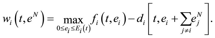Thus, the welfare function of player is given by:

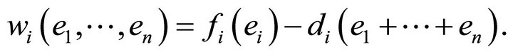(1)

In the noncooperative scenario, each player has to satisfy the environmental constraint:. For each vector he/she has to solve the optimization problem:

More precisely, the problem under consideration is a Nash equilibrium problem, i.e., to find a vector

such that for all one has

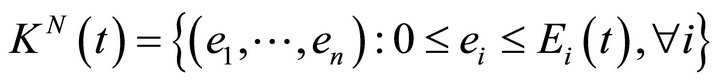
Under the differentiability hypotheses, it is well known (see e.g. [12]) that Nash equilibrium problems are equivalent to variational inequalities. Thus, consider the closed convex set

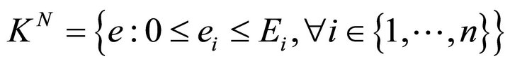
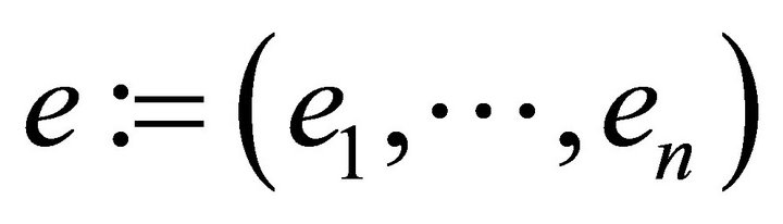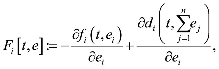
where and let 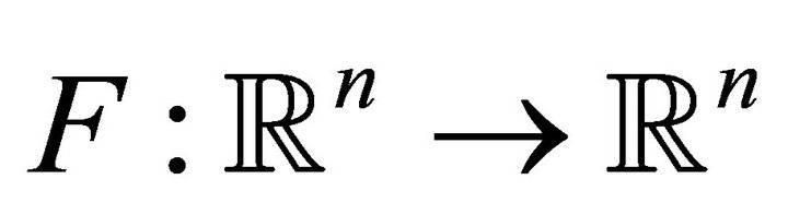be defined by:

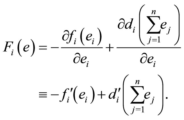
Thus, we can consider the following variational inequality problem: Find

such that

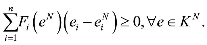(2)

In the sequel we shall refer to the above variational inequality as (NVI). Assume that is a monotone operator i.e.:

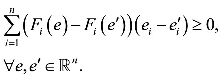(3)

In particular, assume that is strictly monotone in the sense that equality in (3) holds only if. Since is continuous and is compact, the Stampacchia theorem applies and (NVI) is solvable (for a survey on existence theorems for variational inequalities see [13]). Moreover the solution is unique under the strict monotonicity hypothesis.

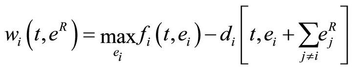
In the umbrella scenario each player still aims to optimize his/her welfare function, for each vector

, but the constraints are satisfied jointly by all players. We are then faced with a generalized Nash equilibrium problem (GNEP), that is the problem of finding such that for all

one has

where

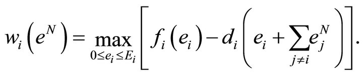
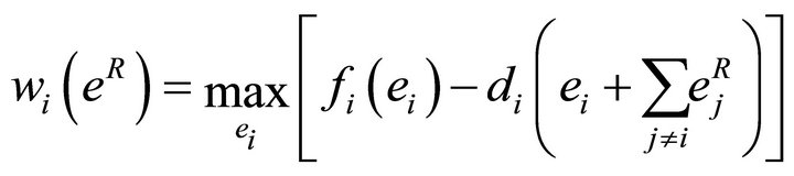
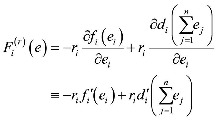
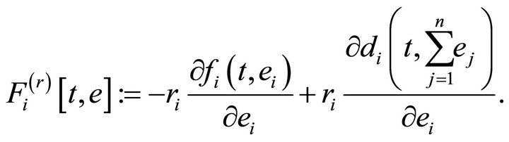
This class of problems was introduced by Rosen in his seminal paper [14] and has been studied quite recently from the point of view of variational inequalities [15]. It is well known that GNEPs have infinite solutions and the problem of selecting certain interesting classes of solutions was already considered by Rosen who introduced the concept of normalized equilibrium. Here we follow and generalize the approach of [15]. Let us fix a vector of positive weights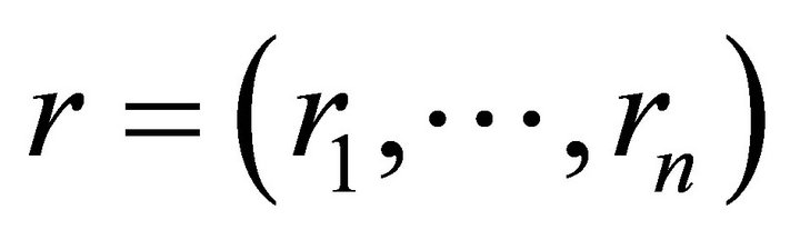, introduce the operator defined by:

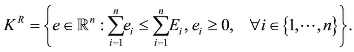
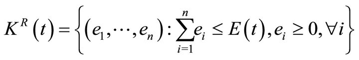
and the closed and convex set:

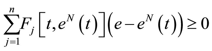
Consider the following variational inequality problem (RVI): Find 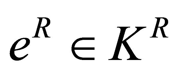such that

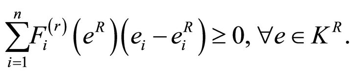(4)

For each fixed vector of weights r this variational inequality admits a unique solution, (since is strictly monotone), which is the normalized Rosen equilibrium corresponding to the given weight. For the economic interpretation of normalized equilibria we refer the interested reader to [2] and to the quoted paper by Rosen. Here we would like to remark that the variational inequality formulation provides a wealth of effective algorithms for the computation of Rosen equilibria.

3. Comparison between Nash and Rosen Equilibrium

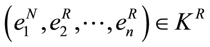
In this section we exploit the variational formulation to compare the total emissions in the two scenarios; we remark that our method does not require the use of Lagrange multipliers. To begin with, let us notice that, if a Rosen equilibrium belongs to the interior ofit follows that, which also implies, i.e. Rosen and Nash equilibrium coincide. Hence, we compare Nash and Rosen total emissions in the following family of subsets of:

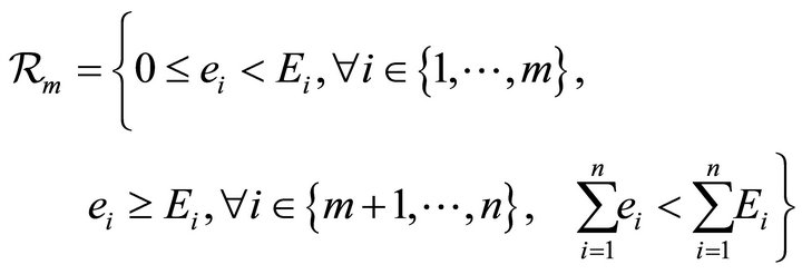
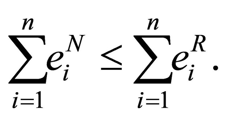
Theorem 1. If, then

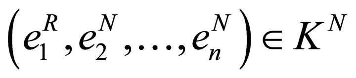
Proof. If the indices for which are not the first, we can always reorder them and consider this case. If, then. If 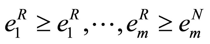as well, it follows that:

(5)

We can prove that (5) continue to hold true if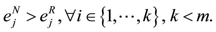

Now, in (4) we can consider as test vector

, and obtain, 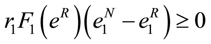, while in (2) we can choose as test vector

, and obtain

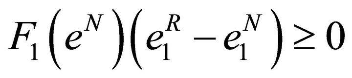
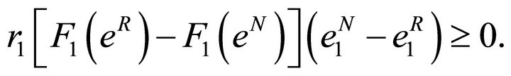
which still holds true after multiplication by. Summing up these two inequalities we get:

(6)

Now we write in detail the first factor:

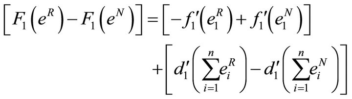
The first expression is negative because 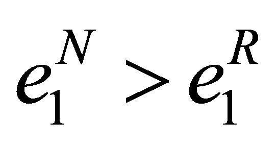and is (strictly) decreasing for all i. Now, let us assumeby contradiction, that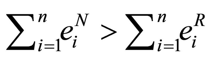. Then, since

is (strictly) decreasing, the second expression is negative as well. As a consequence we would get

, which contradicts (6).

4. Extensions of the Model

Let, and assume that both the welfare functions and the constraints can depend on. More precisely, for each we assume that is such that is measurable , while for almost every (with respect to the Lebesgue measure). Moreover, we assume that the convexity and the monotonicity assumptions that we did in the nonparametric case hold true a.e. in. We are then left with the parametric Nash and Rosen equilibrium problems. The parametric Nash equilibrium problem reads as follows.

For a.e., find:

The parametric Rosen equilibrium problem is: for a.e., find:

where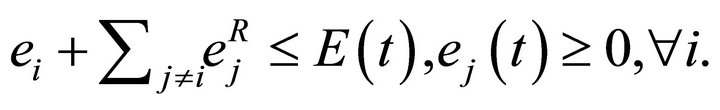

We can then consider the parametric versions of Nash and Rosen variational inequalities. For each consider the two closed and convex subsets of.

where. Moreover, let

Thus, Nash parametric variational inequality is the following problem:

for a.e., find 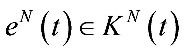such that

(7)

, while Rosen parametric variational inequality reads as follows. For a.e., find with

(8)

Since and are strictly monotone for a.e., it follows that the solution maps and are single valued. To prove the continuity of these maps we state a theorem whose proof can be easly derived along the same line as theorem 2.1 in [6].

Theorem 2. Let be continuous on,;. Moreover, assume that, is strictly concave for all i, and is continuous. Then, (7), (resp. (8)), has a unique solution, (resp. which is continuous on.

In the next theorem we need the following property:

Definition 1. Let. We call T uniformly strongly monotone on, iff such that:

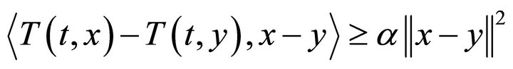(9)

and.

Theorem 3. Let F, (), be uniformly strongly monotone on and Lipschitz continuous on .

Moreover, assume that such that,

(respectively, such that

)

where, (), denotes the projection of a point onto the set, ().

Then, the solution of (7), (of (8) respectively), is Lipschitz continuous on.

For the existence and computation of the geometrical constant see [7].

Now we want to formulate our problems in Lebesgue spaces. For the sake of simplicity we confine ourselves to the Hilbert space.

We shall work under the following set of assumptions:

a) is measurable, , while for almost every.

b).

c) For almost every, is convex with respect to.

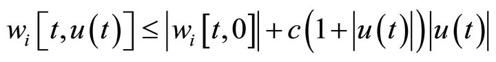
d).

Consider now, for all i, the functionals defined on X:

(10)

We can prove the following theorem.

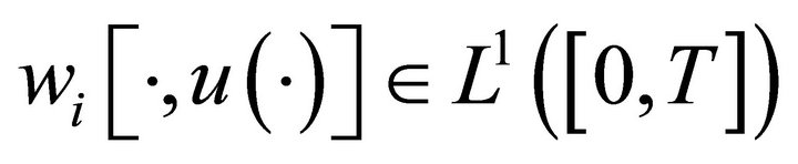
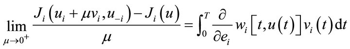
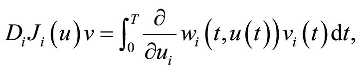
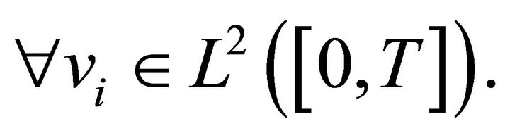
Theorem 4. Assume that the parametric welfare functions satisfiy the assumptions for all i. Then, the functional is well defined in X for each i, and is concave with respect to the variable and Gateaux differentiable in, with respect to. Moreover, its Gateaux derivative is given by:

Proof. Notice first that is well defined due to assumption d). Indeed, for each, there exists, , such that:

hence, we get

a. e. which implies that

.

The concavity of with respect to the variable is an immediate consequence of assumption c). Now we prove that is Gateaux differentiable in X, with respect to, for every. To simplify the notation we write, where. Hence, fix and some direction, and for consider the incremental quotient:

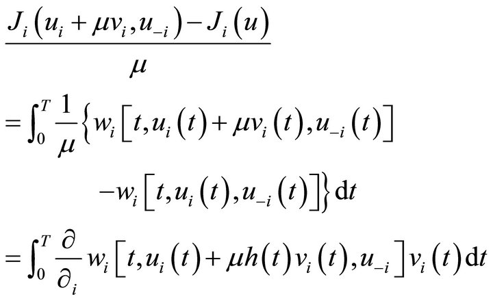
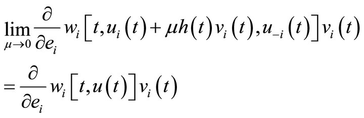
where, a.e.. Now, we have that for a.e.:

Moreover due to the inequality:

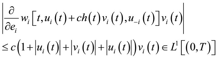
we obtain

by applying Lebesgue convergence theorem.

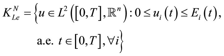
In this framework, the Nash equilibrium problem is to find:

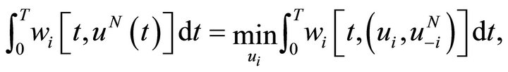
where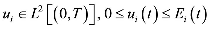, with

.

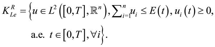
Rosen Equilibrium problem is to find:

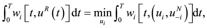
where, and.

Once we have formulated Nash and Rosen equilibrium problems in the Lebesgue space we are in position to write the corresponding two variational inequalities:

Find such that

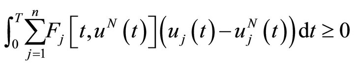(11)

for all, where

Find such that

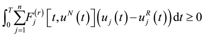(12)

for all, where

5. Conclusion

In this short note we showed how some environmental models recently proposed can be formulated via the variational inequality theory. Moreover, we extended the previous models admitting the possibility that both the operator and the constraints sets depend on a parameter. The variational inequality approach permits the application of some recent geometric-analytic methods ([6,7]) to study the sensitivity of the solution with respect to perturbations of the parameter. At last, we introduced the Lebesgue-space formulation of the problems under study, which, in the last decade, has been very fruitful to study time-dependent and random equilibrium problems (see e.g. [9,11,16] for the approximate computation of statistical quantities related to the solution). In this respect, Inequalities (11) and (12) (and their generalization to probability spaces) are the starting point for a systematic study of environmental problems which we are planning to carry out in the future.

REFERENCES

- M. Breton, G. Zaccour and M. Zahaf, “A Game-Theoretic Formulation of Joint Implementation of Environmental Projects,” European Journal of Operational Research, Vol. 168, No. 1, 2005, pp. 221-239. doi:10.1016/j.ejor.2004.04.026
- M. Tidball and G. Zaccour, “An Environmental Game with Coupling Constraints,” Environmental Modeling and Assessment, Vol. 10, No. 2, 2005, pp. 153-158. doi:10.1007/s10666-005-5254-8
- F. Giannessi and A. Maugeri, Eds., “Variational Inequalities and Network Equilibrium Problems,” Plenum Press, New York, 1995.
- F. Raciti, “Equilibrium Conditions and Vector Variational Inequalities: A Complex Relation,” Journal of Global Optimization, Vol. 40, No. 1-3, 2008, pp. 353-360. doi:10.1007/s10898-007-9202-9
- J. Gwinner and F. Raciti, “Random Equilibrium Problems on Networks,” Mathematical Computer Modelling, Vol. 43, No. 7-8, 2006, pp. 880-891. doi:10.1016/j.mcm.2005.12.007
- A. O. Caruso, A. A. Khan and F. Raciti, “Continuity Results for Some Classes of Variational Inequalities and Applications to Time-Dependent Equilibrium Problems,” Numerical Functional Analysis and Optimization, Vol. 30 No. 11-12, 2009, pp. 1272-1288. doi:10.1080/01630560903381696
- A. Causa and F. Raciti, “Lipschitz Continuity Results for a Class of Variational Inequalities: A Geometric Approach,” Journal of Optimization Theory and Applications, Vol. 145, No. 2, 2010, pp. 235-248. doi:10.1007/s10957-009-9622-4
- A. Causa and F. Raciti, “Some Remarks on the Walras Equilibrium Problem in Lebesgue Spaces,” Optimization Letters, Vol. 5, No. 1, 2011, pp. 99-112. doi:10.1007/s11590-010-0193-y
- J. Gwinner and F. Raciti, “On a Class of Random Variational Inequalities on Random Sets,” Numerical Functional Analysis and Optimization, Vol. 27, No. 5-6, 2006, pp. 619-636.
- J. Gwinner and F. Raciti, “On Monotone Variational Inequalities with Random Data,” Journal of Mathematical Inequalities, Vol. 3, No. 3, 2009, pp. 443-453.
- J. Gwinner and F. Raciti, “Some Equilibrium Problems under Uncertainty and Random Variational Inequalities, Annals of Operations Research, Vol. 200, No. 1, 2012, pp. 299-319. doi:10.1007/s10479-012-1109-2
- P. T. Harker, “Generalized Nash Games and Quasi-Variational Inequalities,” European Journal of Operational Research, Vol. 54, No. 1, 1991, pp. 81-94. doi:10.1016/0377-2217(91)90325-P
- A. Maugeri and F. Raciti, “On Existence Theorems for Monotone and Nonmonotone Variational Inequalities,” Journal of Convex Analysis, Vol. 16, No. 3-4, 2009, pp. 899-911.
- J. B. Rosen, “Existence and Uniqueness of Equilibrium Points for Concave N-Person Games,” Econometrica, Vol. 33, No. 3, 1965, pp. 520-534. doi:10.2307/1911749
- F. Facchinei, A. Fischer and V. Piccialli, “On Generalized Nash Games and Variational Inequalities,” Operations Research Letters, Vol. 35, No. 2, 2007, pp. 159-164. doi:10.1016/j.orl.2006.03.004
- P. Falsaperla, F. Raciti and L. Scrimali, “A Variational Inequality Model of the Spatial Price Network Problem with Uncertain Data,” Optimization and Engineering, Vol. 13, No. 3, 2012, pp. 417-434. doi:10.1007/s11081-011-9158-y