Paper Menu >>
Journal Menu >>
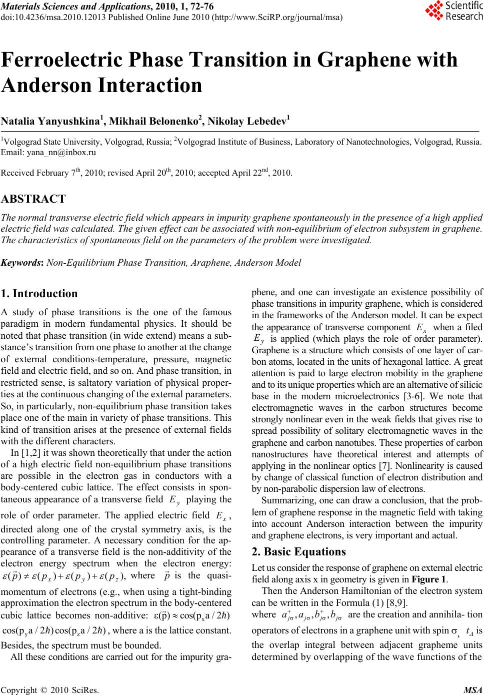 Materials Sciences and Applicatio ns, 2010, 1, 72-76 doi:10.4236/msa.2010.12013 Published Online June 2010 (http://www.SciRP.org/journal/msa) Copyright © 2010 SciRes. MSA Ferroelectric Phase Transition in Graphene with Anderson Interaction Natalia Yanyushkina1, Mikhail Belonenko2, Nikolay Lebedev1 1Volgograd State University, Volgograd, Russia; 2Volgograd Institute of Business, Laboratory of Nanotechnologies, Volgograd, Russia. Email: yana_nn@inbox.ru Received February 7th, 2010; revised April 20th, 2010; accepted April 22nd, 2010. ABSTRACT The normal transverse electric field which appears in impurity graphene spontaneously in the presence of a high applied electric field was calculated. The given effect can be associated with non-equilibrium of electron subsystem in graphene. The characteristics of spontaneous field on the parameters of the problem were investigated. Keywords: Non-Equilibrium Phase Transition, Araphene, Anderson Model 1. Introduction A study of phase transitions is the one of the famous paradigm in modern fundamental physics. It should be noted that phase transition (in wide extend) means a sub- stance’s transition from one phase to another at the change of external conditions-temperature, pressure, magnetic field and electric field, and so on. And phase transition, in restricted sense, is saltatory variation of physical proper- ties at the continuous changing of the external parameters. So, in particularly, non-equilibrium phase transition takes place one of the main in variety of phase transitions. This kind of transition arises at the presence of external fields with the different characters. In [1,2] it was shown theoretically that under the action of a high electric field non-equilibrium phase transitions are possible in the electron gas in conductors with a body-centered cubic lattice. The effect consists in spon- taneous appearance of a transverse field playing the role of order parameter. The applied electric field , directed along one of the crystal symmetry axis, is the controlling parameter. A necessary condition for the ap- pearance of a transverse field is the non-additivity of the electron energy spectrum when the electron energy: y E x E ),()()()( zyx pppp where p is the quasi- momentum of electrons (e.g., when using a tight-binding approximation the electron spectrum in the body-centered cubic lattice becomes non-additive: , where а is the lattice constant. Besides, the spectrum must be bounded. x os(p a(p)c / 2) yz cos(pa / 2)cos(pa / 2) All these conditions are carried out for the impurity gra- phene, and one can investigate an existence possibility of phase transitions in impurity graphene, which is considered in the frameworks of the Anderson model. It can be expect the appearance of transverse component x when a filed E y E is applied (which plays the role of order parameter). Graphene is a structure which consists of one layer of car- bon atoms, located in the units of hexagonal lattice. A great attention is paid to large electron mobility in the graphene and to its unique properties which are an alternative of silicic base in the modern microelectronics [3-6]. We note that electromagnetic waves in the carbon structures become strongly nonlinear even in the weak fields that gives rise to spread possibility of solitary electromagnetic waves in the graphene and carbon nanotubes. These properties of carbon nanostructures have theoretical interest and attempts of applying in the nonlinear optics [7]. Nonlinearity is caused by change of classical function of electron distribution and by non-parabolic dispersion law of electrons. Summarizing, one can draw a conclusion, that the prob- lem of graphene response in the magnetic field with taking into account Anderson interaction between the impurity and graphene electrons, is very important and actual. 2. Basic Equations Let us consider the response of graphene on external electric field along axis x in geometry is given in Figure 1. Then the Anderson Hamiltonian of the electron system can be written in the Formula (1) [8,9]. where ,,, j jjj aabb are the creation and annihila- tion operators of electrons in a graphene unit with spin , t is the overlap integral between adjacent grapheme units determined by overlapping of the wave functions of the  Ferroelectric Phase Transition in Graphene with Anderson Interaction 73 Figure 1. Geometry of a problem grapheme electrons, U is the constant of Coulomb repul- sion of the electros at the same unit; are the creation and annihilation operators of impurity electrons in a graphene spin; + jσjσ d,d is the energy of impurity electrons; U1 is the energy of Coulomb repulsion of impurity elec- trons only. V is the hybridization parameter. The following parameters were estimated by MNDO method [10]: 2 eV, 12 eV, 12 eV, V t U1 U 2 eV. Since the properties of the model described by the Anderson Hamiltonian is sufficiently complex, further we will use the approximation: U→∞ and consider, all mean value is to be spatially homogenous. Note that the approximation U→∞ is well supported by quantum chemical calculations for graphene-like. In this approxima- tion the Hamiltonian (1) can be written as [11,12]. ()kk k H Eps k CC (2) where kk C,C are the creation and annihilation op- erators of elementary excitations (with momentum k and spin σ), and is the spectrum which, according to [11,12], can be presented as: )k(Eps 2 2)1(4))(( )( 2 1 )( Vnnk nkkEps im (3) where V is the hybridization parameter, )( k is the spectrum of graphene electrons determined by the Ham- iltonian , а and are parameters determined from the self-consistency conditions of the problem. h H nim n Note, that dispersion law, which describes graphene properties without taking into account Coulomb repulsion at the same unit, has a following form [13]. y 2 x ap ap (k)14cos(ap)cos( )4cos( ) 33 y (4) where 7.2 eV, a3b/2 , b 0.142 nm is the distance between adjacent carbon atoms in graphene, and ),yx p(pk . According to [11,12], the self-consistency conditions are: We use the average electron method with taking into 1 ()( () () himhyb hjjjjjjjjjjjj jj imjj jjjjjj j hybjjj j j HH HH Ht abbaUaaaabbbb HddddUdddd HVadda ) (1) vv k,v im vv k,v 2 v v vv 2 v2im v 2 2im nAF(E(k)), nBF(E(k)), V A(1) , 2Q (k) E(k) B(1) , 2Q (k) 1 E(k)n(1)((k)n)4(1n)V 2 1 Q(k)((k)n)4(1 n )V 2 , (5) Copyright © 2010 SciRes. MSA  74 Ferroelectric Phase Transition in Graphene with Anderson Interaction account the motion equation can be written as [14]. dp =E dt (6) one can apply:1A Ect , and for low-temperaturecase it is possible to obtain: x 0x x y0yy p =p +Et p =p +Et It should be noted: () () (), () x y xy x Epsp, pEpsp, p υpυp p xy y p Further, we use the average electron method, according to which the current can be expressed as [15]. (())exp() ¥ 0 j= υpt -tdt (7) where j is the density of current, )( t pis the solution of (6) with some initial conditions, which correspond to the energy minimum. In our case, it is necessary to consider the solutions of (8) for four initial conditions (correspond to minimum of ): )( pE 03 xxy y ap=;ap= π;ap= π/;ap=π23 / . Then we should sum up all values for current. It is convenient to represent the dispersion law of gra- phene in the following form: 2 () cos()cos() 1()cos()cos() (2 ) xymn xy m,n ππ mnx yxyxy -π-π εp,p=Ampnp , A= εp,pmpnpdpdp π Finally, in this case: 222 22 22 cos(2)cos() (-1) 33 (-1- ) (1())(1() ) i xmn m,n xy x yx yx mk j= Aπ+π×× mE nEmE ×+nE+mE+nE-mE (8) The transverse field is defined by boundary condi- tions for the given applied filed . Let us assume that a circuit is opened in the x-direction: x E y E 0 x j (9) This condition corresponds to some solve for the trans- verse field: . Equation (9) has two solves: )( yxx EEE 0 ))(1)()(1( )1( 0 , 22 22222 nm xyxy xy mn x mEnEmEnE EmEnm A E (10) The transverse field spontaneously appears in one of two mutually opposite directions at the some values of parameters in the second equation of (10). In this case, we deal with non-equilibrium one-order phase transition. The appearance of the transverse field component represents perhaps the simplest example of self-organization in the impurity graphene. 3. Calculation Results A typical dependence of on , which described by (8), is represented in Figure 2. Dependence of the trans- verse field on the applied field , which deter- mined as non-zero solve of (10) is given in Figure 3 and Figure 4. x jx E x Ey E It worth to note that analogous dependence on the pa- rameter V is weak, and existence of two non-zero solves is more important. One of this solve (smaller in module) is thermodynamically unstable. As might be expected, ac- cording to the numerator of expression (10) increase in the field leads to an increase in the field , due to the y Ex E non-additivity of the electron dispersion. Note the fact that the dependence of the field on is mainly asso- x Ey E ciated with the view of the electron spectrum without interaction (4), and the effects of the interaction of elec- trons with impurities contribute only relatively small corrections. This can also be attributed to the effect is due to non-additivity of the dispersion and less sensitive to the particular type of spectrum. It should be noted that it fol- lows from (10) and Figures 3 and 4 at large can be y E written: yx EE that may be useful in evaluating the field intensities in the experiment. Dependence of a minimal value of the field , at which the transverse field appears, on the at the different is given in Figure 5. y E im n n Note, that the minimal value of is more strongly depends on impurity concentration. It can be associated with reconstruction of the graphene electron spectrum in the presence of impurities. y E The transverse field x E, which is emergent sponta- neously, can be thermodinamically unstanble, as opposite to always stable solve for open circuit in the x-direction = 0. x E We also investigate the stability using the method pro- posed in [1]. We introduct the following function: fixedE tconsEdEjEФ y E xxxx x 0 tan)()( (11) The given function is usually called with synergetic potential and it is the analogue of a thermodynamic potential for non-equilibrium tasks. According to [1], the Copyright © 2010 SciRes. MSA  Ferroelectric Phase Transition in Graphene with Anderson Interaction 75 Figure 2. Dependence of current density on the field Ex, when the field Ey is fixed (Ey = 4.0). All magnitudes are in the non-dimensionless units Figure 3. Dependence of the field Ex on the field E y:(a) ; (b) . All magni- tudes are in the non-dimensionless units 25.0,1.0nim n25.0,5.0nim n stable conditions are: 00 2 2 x xdE Фd dE dФ (12) These formulas mean that in given non-equilibrium situation the function (11) attains its minimum in the stationary state. Thus the function Ф may be regarded as the analogue of a thermodynamic potential for equilibr- ium systems. Dependence of the “potential” Ф on the field for some values of the is presented in Figure 6. It can be seen that the function Ф has the minimum and the maximum. It should be noted, maximum corresponds to a smaller in module solve of Equation (10), and minimum corresponds to a larger in module solve. It means the x Ey E Figure 4. Dependence of the field on the field :(a) ; (b) . All magni- tudes are in the non-dimensionless units x E ,1 n y E 25.0,1.0n im n75.0.0nim Figure 5. Dependence of the minimum on the: (a) ; (b); (c) . All magnitudes are in the non-dimensionless units y Eim n 25.0 n50.0 n75.0 n larger in module solve is stable. Note that dotted branhes in Figure 3 and Figure 4. correspond to the maximum of function Ф (unstable solve), but solid curve and dashed curve correspond to minimum (stable solve). This transition, in which the electric field appears spontaneously, is concerned to ferroelectric type. Though, the transverse field plays the role of the order pa- rameter, and the field x E y E is the analogue of temperature (controlling parameter). The transverse field occurred spontaneously, obviously, can be found by measuring the charge on the capacitor, Copyright © 2010 SciRes. MSA 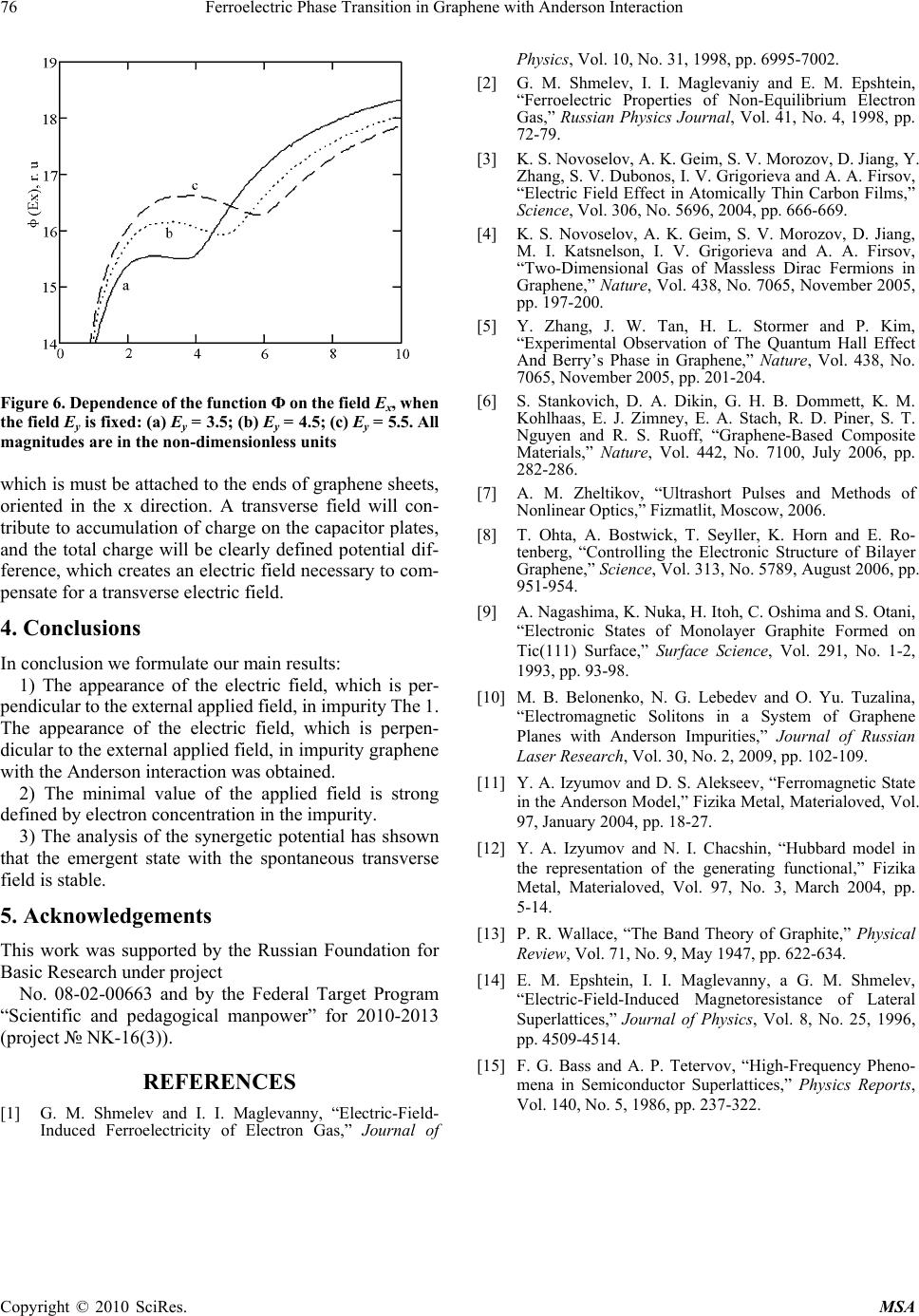 76 Ferroelectric Phase Transition in Graphene with Anderson Interaction Copyright © 2010 SciRes. MSA Figure 6. Dependence of the function Ф on the field Ex, when the field Ey is fixed: (a) Ey = 3.5; (b) Ey = 4.5; (c) Ey = 5.5. All magnitudes are in the non-dimensionless units which is must be attached to the ends of graphene sheets, oriented in the x direction. A transverse field will con- tribute to accumulation of charge on the capacitor plates, and the total charge will be clearly defined potential dif- ference, which creates an electric field necessary to com- pensate for a transverse electric field. 4. Conclusions In conclusion we formulate our main results: 1) The appearance of the electric field, which is per- pendicular to the external applied field, in impurity The 1. The appearance of the electric field, which is perpen- dicular to the external applied field, in impurity graphene with the Anderson interaction was obtained. 2) The minimal value of the applied field is strong defined by electron concentration in the impurity. 3) The analysis of the synergetic potential has shsown that the emergent state with the spontaneous transverse field is stable. 5. Acknowledgements This work was supported by the Russian Foundation for Basic Research under project No. 08-02-00663 and by the Federal Target Program “Scientific and pedagogical manpower” for 2010-2013 (project № NK-16(3)). REFERENCES [1] G. M. Shmelev and I. I. Maglevanny, “Electric-Field- Induced Ferroelectricity of Electron Gas,” Journal of Physics, Vol. 10, No. 31, 1998, pp. 6995-7002. [2] G. М. Shmelev, I. I. Maglevaniy and Е. М. Epshtein, “Ferroelectric Properties of Non-Equilibrium Electron Gas,” Russian Physics Journal, Vol. 41, No. 4, 1998, pp. 72-79. [3] K. S. Novoselov, A. K. Geim, S. V. Morozov, D. Jiang, Y. Zhang, S. V. Dubonos, I. V. Grigorieva and A. A. Firsov, “Electric Field Effect in Atomically Thin Carbon Films,” Science, Vol. 306, No. 5696, 2004, pp. 666-669. [4] K. S. Novoselov, A. K. Geim, S. V. Morozov, D. Jiang, M. I. Katsnelson, I. V. Grigorieva and A. A. Firsov, “Two-Dimensional Gas of Massless Dirac Fermions in Graphene,” Nature, Vol. 438, No. 7065, November 2005, pp. 197-200. [5] Y. Zhang, J. W. Tan, H. L. Stormer and P. Kim, “Experimental Observation of The Quantum Hall Effect And Berry’s Phase in Graphene,” Nature, Vol. 438, No. 7065, November 2005, pp. 201-204. [6] S. Stankovich, D. A. Dikin, G. H. B. Dommett, K. M. Kohlhaas, E. J. Zimney, E. A. Stach, R. D. Piner, S. T. Nguyen and R. S. Ruoff, “Graphene-Based Composite Materials,” Nature, Vol. 442, No. 7100, July 2006, pp. 282-286. [7] A. M. Zheltikov, “Ultrashort Pulses and Methods of Nonlinear Optics,” Fizmatlit, Moscow, 2006. [8] T. Ohta, A. Bostwick, T. Seyller, K. Horn and E. Ro- tenberg, “Controlling the Electronic Structure of Bilayer Graphene,” Science, Vol. 313, No. 5789, August 2006, pp. 951-954. [9] A. Nagashima, K. Nuka, H. Itoh, C. Oshima and S. Otani, “Electronic States of Monolayer Graphite Formed on Tic(111) Surface,” Surface Science, Vol. 291, No. 1-2, 1993, pp. 93-98. [10] M. B. Belonenko, N. G. Lebedev and O. Yu. Tuzalina, “Electromagnetic Solitons in a System of Graphene Planes with Anderson Impurities,” Journal of Russian Laser Research, Vol. 30, No. 2, 2009, pp. 102-109. [11] Y. A. Izyumov and D. S. Аlekseev, “Ferromagnetic State in the Anderson Model,” Fizika Metal, Materialoved, Vol. 97, January 2004, pp. 18-27. [12] Y. A. Izyumov and N. I. Chacshin, “Hubbard model in the representation of the generating functional,” Fizika Metal, Materialoved, Vol. 97, No. 3, March 2004, pp. 5-14. [13] P. R. Wallace, “The Band Theory of Graphite,” Physical Review, Vol. 71, No. 9, May 1947, pp. 622-634. [14] E. M. Epshtein, I. I. Maglevanny, a G. M. Shmelev, “Electric-Field-Induced Magnetoresistance of Lateral Superlattices,” Journal of Physics, Vol. 8, No. 25, 1996, pp. 4509-4514. [15] F. G. Bass and A. P. Tetervov, “High-Frequency Pheno- mena in Semiconductor Superlattices,” Physics Reports, Vol. 140, No. 5, 1986, pp. 237-322. |