Journal of Minerals & Materials Characterization & Engineering, Vol. 10, No.10, pp.875-886, 2011
jmmce.org Printed in the USA. All rights reserved
875
Prediction of Weld Bead Geometry in Plasma Arc Welding using Factorial
Design Approach
1*
K. Siva Prasad,
2
Ch.Srinivasa Rao,
2
D.Nageswara Rao
1
Department of Mechanical Engineering,
Anil Neeerukonda Institute of Technology & Sciences, Visakhapatnam, India.
2
Department of Mechanical Engineering, Andhra University, Visakhapatnam, India
*Corresponding Author : [e-mail]
ABSTRACT
The effect of various process parameters like welding current, torch height, welding speed
and plasma gas flow rate on front melting width, back melting width and weld reinforcement
of plasma arc welding on aluminum alloy is investigated by using factorial design approach.
Variable polarity plasma arc welding is used for welding aluminum alloy. Trail experiments
are conducted and the limits of the input process parameters are decided. Two levels and four
input process parameters are chosen and experiments are conducted as per typical design
matrix considering full factorial design. Total sixteen experiments are conducted and output
responses are measured. The coefficients are calculated by using regression analysis and the
mathematical models are constructed. By using the mathematical models the main and
interaction effect of various process parameters on weld quality is studied.
Key Words: Plasma Arc Welding, Factorial Design, , Regression Analysis, Welding current,
Welding speed, Torch height, Plasma gas flow rate, Front Melting Width, Back Melting
Width, Weld Reinforcement.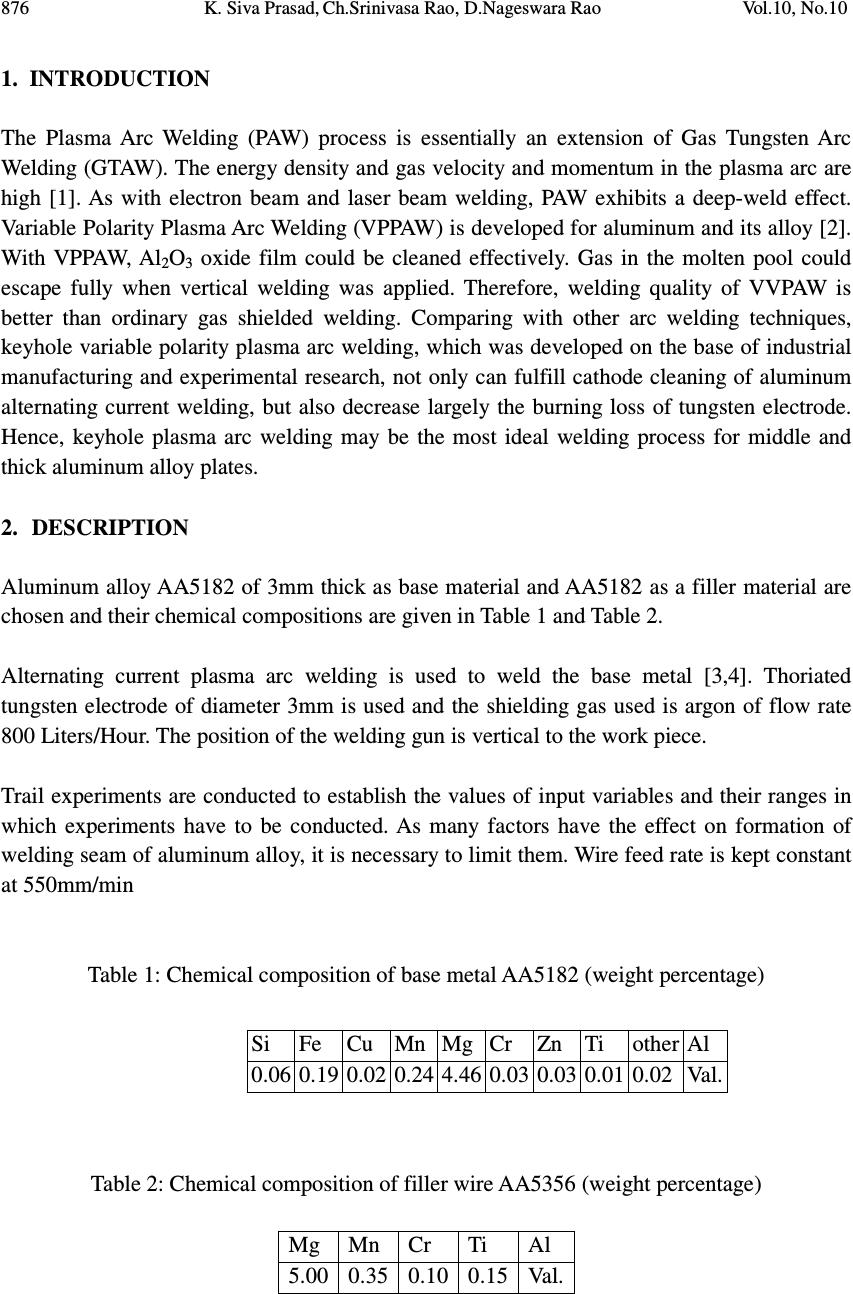

876 K. Siva Prasad, Ch.Srinivasa Rao, D.Nageswara Rao Vol.10, No.10
1. INTRODUCTION
The Plasma Arc Welding (PAW) process is essentially an extension of Gas Tungsten Arc
Welding (GTAW). The energy density and gas velocity and momentum in the plasma arc are
high [1]. As with electron beam and laser beam welding, PAW exhibits a deep-weld effect.
Variable Polarity Plasma Arc Welding (VPPAW) is developed for aluminum and its alloy [2].
With VPPAW, Al
2
O
3
oxide film could be cleaned effectively. Gas in the molten pool could
escape fully when vertical welding was applied. Therefore, welding quality of VVPAW is
better than ordinary gas shielded welding. Comparing with other arc welding techniques,
keyhole variable polarity plasma arc welding, which was developed on the base of industrial
manufacturing and experimental research, not only can fulfill cathode cleaning of aluminum
alternating current welding, but also decrease largely the burning loss of tungsten electrode.
Hence, keyhole plasma arc welding may be the most ideal welding process for middle and
thick aluminum alloy plates.
2. DESCRIPTION
Aluminum alloy AA5182 of 3mm thick as base material and AA5182 as a filler material are
chosen and their chemical compositions are given in Table 1 and Table 2.
Alternating current plasma arc welding is used to weld the base metal [3,4]. Thoriated
tungsten electrode of diameter 3mm is used and the shielding gas used is argon of flow rate
800 Liters/Hour. The position of the welding gun is vertical to the work piece.
Trail experiments are conducted to establish the values of input variables and their ranges in
which experiments have to be conducted. As many factors have the effect on formation of
welding seam of aluminum alloy, it is necessary to limit them. Wire feed rate is kept constant
at 550mm/min
Table 1: Chemical composition of base metal AA5182 (weight percentage)
Table 2: Chemical composition of filler wire AA5356 (weight percentage)
Mg Mn Cr Ti Al
5.00 0.35 0.10 0.15 Val.
Si Fe Cu Mn Mg Cr Zn Ti other Al
0.06 0.19 0.02 0.24 4.46 0.03 0.03 0.01 0.02 Val.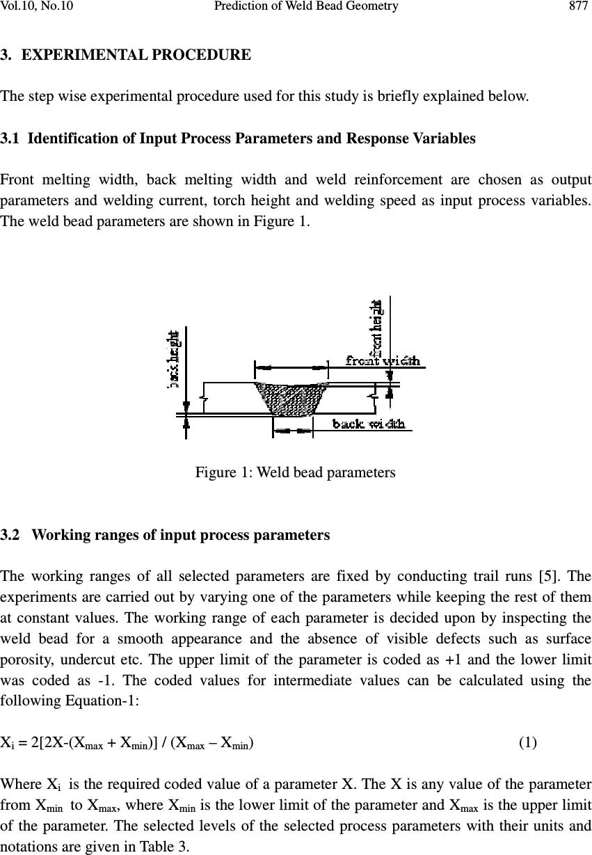

Vol.10, No.10 Prediction of Weld Bead Geometry 877
3. EXPERIMENTAL PROCEDURE
The step wise experimental procedure used for this study is briefly explained below.
3.1 Identification of Input Process Parameters and Response Variables
Front melting width, back melting width and weld reinforcement are chosen as output
parameters and welding current, torch height and welding speed as input process variables.
The weld bead parameters are shown in Figure 1.
Figure 1: Weld bead parameters
3.2 Working ranges of input process parameters
The working ranges of all selected parameters are fixed by conducting trail runs [5]. The
experiments are carried out by varying one of the parameters while keeping the rest of them
at constant values. The working range of each parameter is decided upon by inspecting the
weld bead for a smooth appearance and the absence of visible defects such as surface
porosity, undercut etc. The upper limit of the parameter is coded as +1 and the lower limit
was coded as -1. The coded values for intermediate values can be calculated using the
following Equation-1:
X
i
= 2[2X-(X
max
+ X
min
)] / (X
max
– X
min
) (1)
Where X
i
is the required coded value of a parameter X. The X is any value of the parameter
from X
min
to X
max
, where X
min
is the lower limit of the parameter and X
max
is the upper limit
of the parameter. The selected levels of the selected process parameters with their units and
notations are given in Table 3.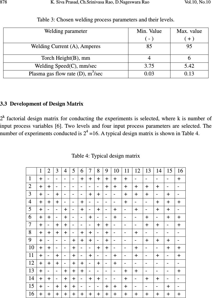

878 K. Siva Prasad, Ch.Srinivasa Rao, D.Nageswara Rao Vol.10, No.10
Table 3: Chosen welding process parameters and their levels.
3.3 Development of Design Matrix
2
k
factorial design matrix for conducting the experiments is selected, where k is number of
input process variables [6]. Two levels and four input process parameters are selected. The
number of experiments conducted is 2
4
=16. A typical design matrix is shown in Table 4.
Table 4: Typical design matrix
1 2 3 4 5 6 7 8 9 10 11 12 13 14 15 16
1 + - - - - + + + + + + - - - - +
2 + + - - - - - - + + + + + + - -
3 + - + - - - + + - - + + + - + -
4 + + + - - + - - - - + - - + + +
5 + - - + - + - + - + - + - + + -
6 + + - + - - + - - + - - + - + +
7 + - + + - - - + + - - - + + - +
8 + + + + - + + - + - - + - - - -
9 + - - - + + + - + - - - + + + -
10 + + - - + - - + + - - + - - + +
11 + - + - + - + - - + - + - + - +
12 + + + - + + - + - + - - - - - -
13 + - - + + + - - - - + + - - - +
14 + + - + + - + + - - + - + + - -
15 + - + + + - - - + + + - - - + -
16 + + + + + + + + + + + + + + + +
Welding parameter Min. Value
( - )
Max. value
( + )
Welding Current (A), Amperes 85 95
Torch Height(B), mm 4 6
Welding Speed(C), mm/sec 3.75 5.42
Plasma gas flow rate (D), m
3
/sec 0.03 0.13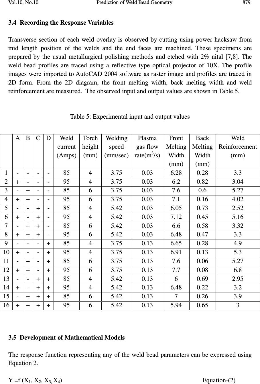

Vol.10, No.10 Prediction of Weld Bead Geometry 879
3.4 Recording the Response Variables
Transverse section of each weld overlay is observed by cutting using power hacksaw from
mid length position of the welds and the end faces are machined. These specimens are
prepared by the usual metallurgical polishing methods and etched with 2% nital [7,8]. The
weld bead profiles are traced using a reflective type optical projector of 10X. The profile
images were imported to AutoCAD 2004 software as raster image and profiles are traced in
2D form. From the 2D diagram, the front melting width, back melting width and weld
reinforcement are measured. The observed input and output values are shown in Table 5.
Table 5: Experimental input and output values
3.5 Development of Mathematical Models
The response function representing any of the weld bead parameters can be expressed using
Equation 2.
Y =f (X
1
, X
2
, X
3,
X
4
) Equation-(2)
A B C D Weld
current
(Amps)
Torch
height
(mm)
Welding
speed
(mm/sec)
Plasma
gas flow
rate(m
3
/s)
Front
Melting
Width
(mm)
Back
Melting
Width
(mm)
Weld
Reinforcement
(mm)
1 - - - - 85 4 3.75 0.03 6.28 0.28 3.3
2 + - - - 95 4 3.75 0.03 6.2 0.82 3.04
3 - + - - 85 6 3.75 0.03 7.6 0.6 5.27
4 + + - - 95 6 3.75 0.03 7.1 0.16 4.02
5 - - + - 85 4 5.42 0.03 6.05 0.73 2.52
6 + - + - 95 4 5.42 0.03 7.12 0.45 5.16
7 - + + - 85 6 5.42 0.03 6.6 0.58 3.32
8 + + + - 95 6 5.42 0.03 6.48 0.47 3.3
9 - - - + 85 4 3.75 0.13 6.65 0.28 4.9
10 + - - + 95 4 3.75 0.13 6.91 0.13 5.3
11 - + - + 85 6 3.75 0.13 7.6 0.06 5.27
12 + + - + 95 6 3.75 0.13 7.7 0.08 6.8
13 - - + + 85 4 5.42 0.13 6 0.69 2.95
14 + - + + 95 4 5.42 0.13 6.48 0.22 3.2
15 - + + + 85 6 5.42 0.13 7 0.26 3.9
16 + + + + 95 6 5.42 0.13 5.94 0.65 3

880 K. Siva Prasad, Ch.Srinivasa Rao, D.Nageswara Rao Vol.10, No.10
Where Y is the response i.e. output parameters and X
1
, X
2
, X
3
, X
4
are the input variables [9].
The first step is to find suitable approximation for the true function of relationship between Y
and the set of independent variables. Usually, a low-order polynomial in some region of the
independent variables is employed. If the response is well modeled by a linear function of
the independent variables then the approximating function is the first order model as shown
in Equation 3.
Y=K+AX
1
+BX
2
+CX
3
+DX
4
+ABX
1
X
2
+ACX
1
X
3
+ADX
1
X
4
+BCX
2
X
3
+BDX
2
X
4
+
CDX
3
X
4
+ABCX
1
X
2
X
3
+ABDX
1
X
2
X
4
+ACDX
1
X
3
X
4
+BCDX
2
X
3
X
4
+
ABCDX
1
X
2
X
3
X
4
Equation (3)
Where A, B, C, D are regression coefficeints and K indicate the noise.
The regression coefficients are calculated using the design matrix shown in Table 4.
The actual mathematical models for Front Melting Width, Back Melting Width and Weld
Reinforcement are represented in Equations 4, 5 & 6 respectively.
Front Melting Width (FMW)
FMW=6.7318+0.0093X
1
+0.2706X
2
-0.2731X
3
+0.0531X
4
-0.2068X
1
X
2
+0.0368X
1
X
3
-
0.0743X
1
X
4
-0.1868X
2
X
3
-0.0331X
2
X
4
-0.1193X
3
X
4
-0.0968X
1
X
2
X
3
-0.0431X
1
X
2
X
4
-
0.1168X
1
X
3
X
4
+0.1018X
2
X
3
X
4
-0.000625X
1
X
2
X
3
X
4
Equation (4)
Back Melting Width (BMW)
BMW =0.37+0.0025X
1
-0.08X
2
+0.13625X
3
-0.07375X
4
+0.0475X
1
X
2
-0.06125X
1
X
3
-
0.02875X
1
X
4
+0.06375X
2
X
3
+0.04625X
2
X
4
+0.0225X
3
X
4
+0.08125X
1
X
2
X
3
+
0.08125X
1
X
2
X
4
+0.0675X
1
X
3
X
4
-0.03X
2
X
3
X
4
+0.005X
1
X
2
X
3
X
4
Equation (5)
Weld Reinforcement (WR)
WR =4.0781+0.1493X
1
+0.2818X
2
-0.6606X
3
+ 0.3368X
4
-0.2293X
1
X
2
+0.0968X
1
X
3
+
0.106X
1
X
4
-0.3206X
2
X
3
+0.0456X
2
X
4
-0.4931X
3
X
4
-0.2468X
1
X
2
X
3
+0.2268X
1
X
2
X
4
-
0.4193X
1
X
3
X
4
+0.1806X
2
X
3
X
4
-0.0381X
1
X
2
X
3
X
4
Equation (6)
4. RESULTS & DISCUSSION
Graphs 2, 3, 4 represents the scatter diagram indicated how the experimental values and
predicted values (Non-linear model values) vary. Variation of Front melting width, Back
melting width and weld reinforcement with welding current, Torch height, welding speed,
Plasma gas flow rate are shown in graphs 5,6,7,8. Comparisons of experimental and predicted
values are shown in Table 6.

Vol.10, No.10 Prediction of Weld Bead Geometry 881
Table 6: Comparison of experimental and predicted values
5.5
6
6.5
7
7.5
8
6.2 6.4 6.6 6.877.2
ACTUAL VALUES(mm)
PREDICTED VALUES(mm)
FRONT MELTING WIDTH
Figure 2: Scatter plot for Front melting width
Front Melting Width(mm) Back Melting Width (mm) Weld Reinforcement (mm)
Experimental
value
Predicted
value
Experimental
value
Predicted
value
Experimental
value
Predicted
value
6.28 6.575298 0.28 0.375313 3.3 3.855756
6.2 6.642652 0.82 0.455938 3.04 3.913244
7.6 7.049802 0.6 0.249063 5.27 4.434619
7.1 6.980148 0.16 0.297188 4.02 4.263281
6.05 6.408977 0.73 0.528125 2.52 3.436994
7.12 6.619773 0.45 0.474375 5.16 3.914806
6.6 6.694023 0.58 0.44125 3.32 3.718831
6.48 6.671327 0.47 0.43375 3.3 3.740069
6.65 6.727302 0.28 0.310625 4.9 4.365094
6.91 6.800148 0.13 0.289375 5.3 4.615306
7.6 7.139198 0.06 0.20625 5.27 4.776331
7.7 7.032252 0.08 0.23125 6.8 5.043569
6 6.449023 0.69 0.468438 2.95 3.563056
6.48 6.548827 0.22 0.377813 3.2 3.833344
7 6.773577 0.26 0.370938 3.9 3.876919
5.94 6.596473 0.65 0.410313 3 3.898381

882 K. Siva Prasad, Ch.Srinivasa Rao, D.Nageswara Rao Vol.10, No.10
0.1
0.2
0.3
0.4
0.5
0.6
0.1 0.2 0.3 0.4 0.5 0.6
ACTUAL VALUES(mm)
PREDICTED VALUES(mm)
BACK MELTING WIDTH
Figure 3: Scatter plot for Back melting width
2
3
4
5
6
7
8
2 3 4 5 6 78
ACTUAL VALUES(mm)
PREDICTED VALUES(mm)
WELD REINFORCEMENT
Figure 4: Scatter plot for Weld Reinforcement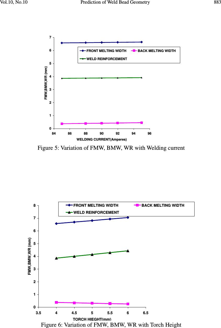

Vol.10, No.10 Prediction of Weld Bead Geometry 883
0
1
2
3
4
5
6
7
84 86 88 90 92 94 96
WELDING CURRENT(Amperes)
FMW,BMW,WR (mm)
FRONT MELTING WIDTHBACK MELTING WIDTH
WELD REINFORCEMENT
Figure 5: Variation of FMW, BMW, WR with Welding current
0
1
2
3
4
5
6
7
8
3.5 4 4.5 5 5.5 66.5
TORCH HIEGHT(mm)
FMW,BMW,WR (mm)
FRONT MELTING WIDTHBACK MELTING WIDTH
WELD REINFORCEMENT
Figure 6: Variation of FMW, BMW, WR with Torch Height

884 K. Siva Prasad, Ch.Srinivasa Rao, D.Nageswara Rao Vol.10, No.10
0
1
2
3
4
5
6
7
3.5 4 4.55 5.5
WELDING SPEED(mm/sec)
FME,BME,WR(mm)
FRONT MELTING WIDTHBACK MELTING WIDTH
WELD REINFORCEMENT
Figure 7: Variation of FMW, BMW, WR with Welding Speed
0
1
2
3
4
5
6
7
8
0.02 0.04 0.06 0.080.10.12 0.14
PLASMA GAS FLOW RATE(m3/sec)
FMW,BMW,WR(mm)
FRONT MELTING WIDTHBACK MELTING WIDTH
WELD REINFORCEMENT
Figure 8: Variation of FMW, BMW, WR with Plasma gas flow rate

Vol.10, No.10 Prediction of Weld Bead Geometry 885
5. CONCLUSIONS
From the experimentation results and developed mathematical models the following
observations are made.
1. The experimental and predicted values are well with in the limits; however there is
some variation in the experimental and predicted values because we had considered
only four input process parameters and two levels in the present paper. The accuracy
of the predicted values can be improved by considering more input process
parameters and more levels.
2. By keeping Torch height and welding speed, Plasma gas flow rate constant and
increasing welding current, Front melting width, Back melting width and weld
reinforcement decreases.
3. By keeping welding current, welding speed, plasma gas flow rate constant and
increasing Torch height, Front melting width and Weld Reinforcement increases
where as Back Melting width decreases.
4. By keeping welding current, Torch height, plasma gas flow rate constant and
increasing welding speed, Front melting width and Weld Reinforcement decreases
where as Back Melting width increases.
5. By keeping welding current, Torch height, welding speed constant and increasing
plasma gas flow rate, Front melting width and Weld Reinforcement decreases
where as Back melting width increases.
6. Because of the complexity in the input parameters the present work is limited to
four parameters variation and its influence on Front melting width, Back melting
width and Weld reinforcement. However there are other factors like wire feed
rate, flow rate of shielding gas etc which also influence the weld quality are kept
constant.
7. In the present paper we had taken only factors and two levels of the input variables;
however for better results more input process parameters and more levels should be
condidered.
ACKNOWLEDGEMETS
We extend our sincere thanks to Shri. R.Gopala Krishna, Director (Technical) , M/s Metallic
Bellows (I) Pvt Ltd, Chennai, India for his support in carrying out the experimentation work .
We also thank all the people who helped us in preparing this paper.
REFERENCES
[1] Howard Cary. B, 1979, Modern Welding Technology, Prentice Hall Inc, Englewood
Cliffs, NJ.
[2] H.X.Wang, Y.H.Wei, C.L.Yang, 2007, Numerical simulation of variable polarity
vertical-up plasma arc welding, J. Computational Materials Science, 38,pp.571-
587.

886 K. Siva Prasad, Ch.Srinivasa Rao, D.Nageswara Rao Vol.10, No.10
[3] Roberts DK, Wells AA, 1954, Fusion welding of aluminum alloys Br, Weld J, 12:
pp.553-559.
[4] ASM Handbook, 1993, welding, brazing and soldering, vol.6.ASM, USA.
[5] V.K.Guptha, R.S.Parmar, 1989, Fractional factorial technique to predict dimensions
of the weld bead in automatic submerged arc welding, J. Inst.Eng. (India), pp.67-70.
[6] G. Cohran, M. Cox, 1963, Experimental Designs, Asia Publishing House, India.
[7] Nouri M, Abdollah-zadehy A, Malek F, 2007, Effect of welding parameters on
dilution and weld bead geometry in cladding. J Mater Sci Technol, 23(6), pp.
817-822.
[8] J.P.Ganjigatti, D.K.Prathhar, A.Roy Choudary, 2008,Modeling of the MIG welding
Process using stastical approaches IntJ Adv Manuf Technol, 35, pp. 1166-1190.
[9] Montgomery dc, 1997, Design and analysis of Experiments, 4th edition, Wiley,
NewYork.