Paper Menu >>
Journal Menu >>
 Journal of Minerals & Materials Characterization & Engineering, Vol. 9, No.5, pp.427-454, 2010 jmmce.org Printed in the USA. All rights reserved 427 Finite Elements in the Solution of Continuum Field Problems Chukwutoo Christopher Ihueze Department of Industrial/ Production Engineering Nnamdi Azikiwe University Awka, Nigeria Email: ihuezechukwutoo @yahoo.com ABSTRACT A finite element functional solution procedure was presented employing variational calculus. The Functionals of field continuum were developed on adoption of Euler minimum integral theorem and finite element procedures on Laplace model. The elements functionals minimization resulted to series of partial differential equations describing the variation of the function of interest at various discrete nodal points. The assembly of the partial differential equations gave a unifying algebraic system of equation was solved for the unique solutions of the function. To simulate the finite element model, boundary conditions of temperature field was assumed. The solution and post processing of FEM of this study showed that once the stiffness matrix of a continuum is established and the boundary conditions specified the continuum is solved uniquely. Regression method was used to establish the error associated with FEM results and to establish a simple prediction model for environmental temperatures. The procedure of this study presented the basis for insulation design for solid, hollow or shell pipes in fluid transport design in oil and gas transport system. The finite element method evaluated the temperature distribution of the region to serve as a guide in quantifying quantity of heat to the environment from the transit fluid. The error of FEM prediction was estimated at 0.006 and the coefficient of determination for goodness of regression fit is estimated as 0.99999. This study also presents an approximate procedure for processing polar systems as rectangular systems by using the circumference of the circular section as one dimensional independent variable and the difference between the inner and outer radius (thickness) as the second i n d ependent variable. Keywords: Calculus of variation, functional, finite element, continuum, field problems, boundary conditions.  Vol.9, No.5 Finite Elements in the Solution of Continuum Field Problems 428 1. INTRODUCTION The essence of this work is to use a simple bounded region to present a procedure to solve functional problems in fluid transport piping system. A finite element functional solution procedure was presented using variational calculus. Mechanics field problems of heat and mass transfer and fluid flow problems in oil and gas industries is intended to be solved following the formulations of this article. Fluid mechanics problems can be studied by isolating a discrete domain with boundary values such as fluids within shelled pipes in which boundary conditions are known. The functional approach expects the flow function to be approximate to known field phenomenon, such as wave phenomenon, , diffusion phenomenon and potential phenomenon, though, some complex phenomena of engineering sciences may be a combination of the above phenomena [1]. An immense number of analytical solutions for conduction heat-transfer problems has been accumulated in the literature over the years past. Even so, in many practical situations the geometry or boundary conditions are such that an analytical solution has not been obtained at all, or if the solution has been developed, it involves such a complex series solution that numerical evaluation becomes exceedingly difficult [2]. However, presently the most fruitful approach to the problem is one based on finite different techniques, the basic principles of which are outlined in [3, 4, 5, and 6]. But because of the short falls of finite difference method the major objective of this article is to present the finite element method, as the most elegant approach of solving function such as the temperature distribution in a medium. Finite element approach is suited to solving partial differential equation so that this work used the finite element approach to develop the partial differential equations of the function at the discrete nodes, and as such the values of the function at the boundary nodes must be known, may be from the field data. In this study linear triangular element is used to discretize the field domain or the mathematical model representing the function, and the following the variational principle and Euler minimum integral theorem to arrive at the elements equations. The elements equations are then added in a finite element format called assembly and the system of the equations solved after the application of boundary conditions to obtain the value of the function that minimizes the functional at the stationary points. The procedure is analogous to Raleigh – Ritz method for stationary total potential applied to elastic problems [7]. Above all, Most Quasi – harmonic field phenomenon are represented by either the partial derivatives of the function or by the well known Laplace and Poisson’s equation [8]. The velocities, temperatures and densities of fluids in oil and gas pipelines are expected to be known at various sections of transport line as the mentioned variables determine efficiency of the transportation unit. 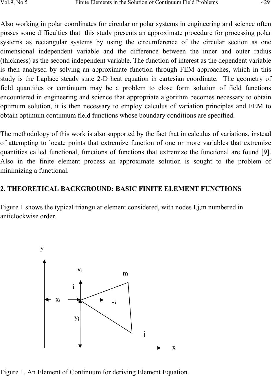 Vol.9, No.5 Finite Elements in the Solution of Continuum Field Problems 429 Also working in polar coordinates for circular or polar systems in engineering and science often posses some difficulties that this study presents an approximate procedure for processing polar systems as rectangular systems by using the circumference of the circular section as one dimensional independent variable and the difference between the inner and outer radius (thickness) as the second independent variable. The function of interest as the dependent variable is then analysed by solving an approximate function through FEM approaches, which in this study is the Laplace steady state 2-D heat equation in cartesian coordinate. The geometry of field quantities or continuum may be a problem to close form solution of field functions encountered in engineering and science that appropriate algorithm becomes necessary to obtain optimum solution, it is then necessary to employ calculus of variation principles and FEM to obtain optimum continuum field functions whose boundary conditions are specified. The methodology of this work is also supported by the fact that in calculus of variations, instead of attempting to locate points that extremize function of one or more variables that extremize quantities called functional, functions of functions that extremize the functional are found [9]. Also in the finite element process an approximate solution is sought to the problem of minimizing a functional. 2. THEORETICAL BACKGROUND: BASIC FINITE ELEMENT FUNCTIONS Figure 1 shows the typical triangular element considered, with nodes I,j,m numbered in anticlockwise order. Figure 1. An Element of Continuum for deriving Element Equation. i m j xi yi vi y x ui 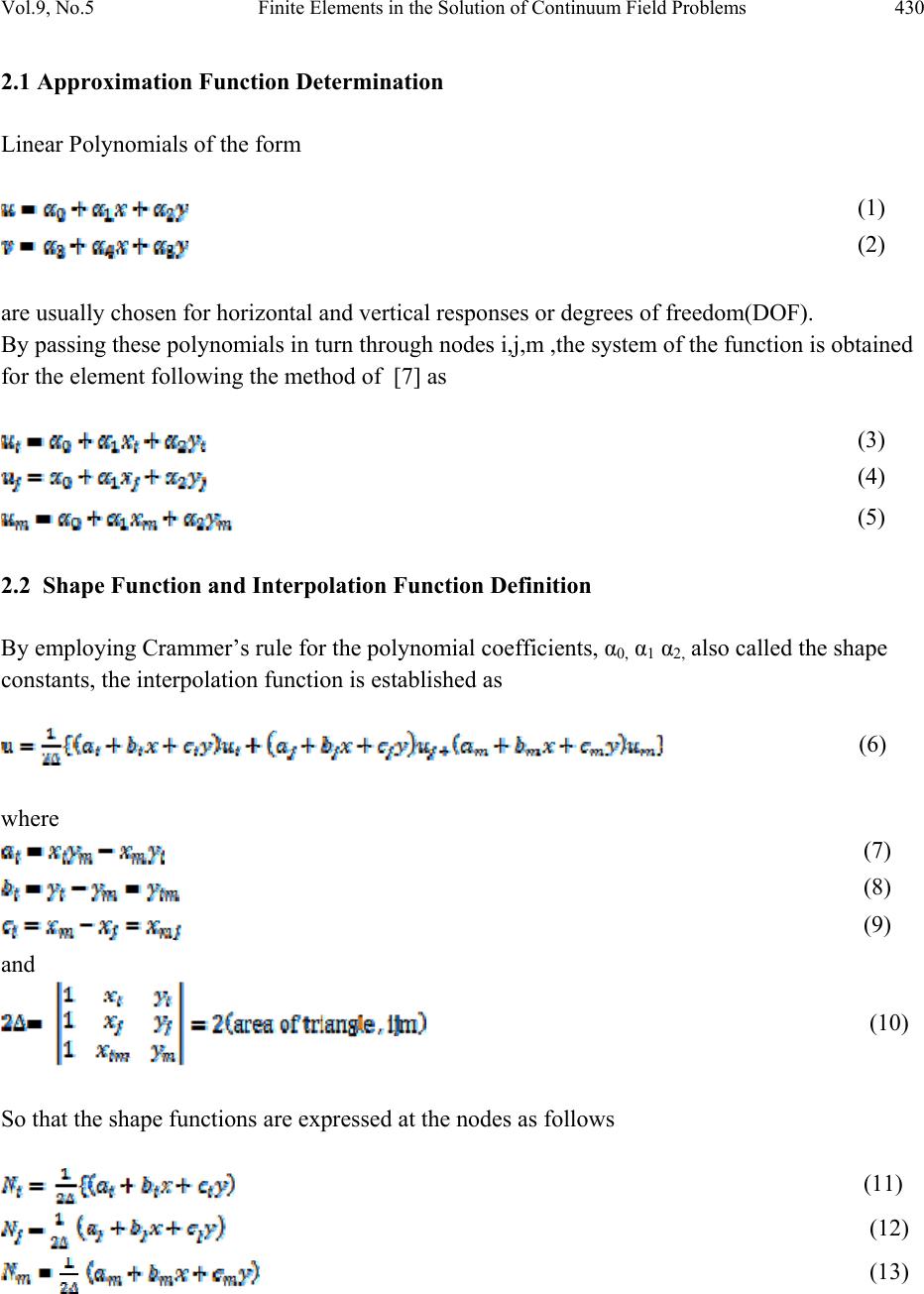 Vol.9, No.5 Finite Elements in the Solution of Continuum Field Problems 430 2.1 Approximation Function Determination Linear Polynomials of the form (1) (2) are usually chosen for horizontal and vertical responses or degrees of freedom(DOF). By passing these polynomials in turn through nodes i,j,m ,the system of the function is obtained for the element following the method of [7] as (3) (4) (5) 2.2 Shape Function and Interpolation Function Definition By employing Crammer’s rule for the polynomial coefficients, α0, α1 α2, also called the shape constants, the interpolation function is established as (6) where (7) (8) (9) and (10) So that the shape functions are expressed at the nodes as follows (11) (12) (13)  Vol.9, No.5 Finite Elements in the Solution of Continuum Field Problems 431 and interpolation function expressed as (14) 2.3 Basic Field Equations and Approximating Functionals [8] Presented the general equation governing quasi-harmonic field functions as + (15) While the theorem of Euler presented by [10] states that if the integral (16) is to be minimized, then the necessary and sufficient condition for this minimum to be reached is that the unknown function u (x, y, z) should satisfy the following differential equation + + (17) within the same region, provided u satisfies the same boundary conditions in both cases, where u = unknown function assumed to be single valued within the region = specified functions of x, y, z x, y, z = space variables The equivalent formulation to that of equation (3) is the requirement that the volume integral given below and taken over the whole region, should be, (18) 3. FORMATION OF FUNCTIONAL OF TWO DIMENSIONAL FIELD FUNCTIONS The functions that can be approximated by two dimensional Laplace equations such as the two dimensional steady state heat transfer problem with constant thermal conductivity are said to be governed by the equation [2] (19) 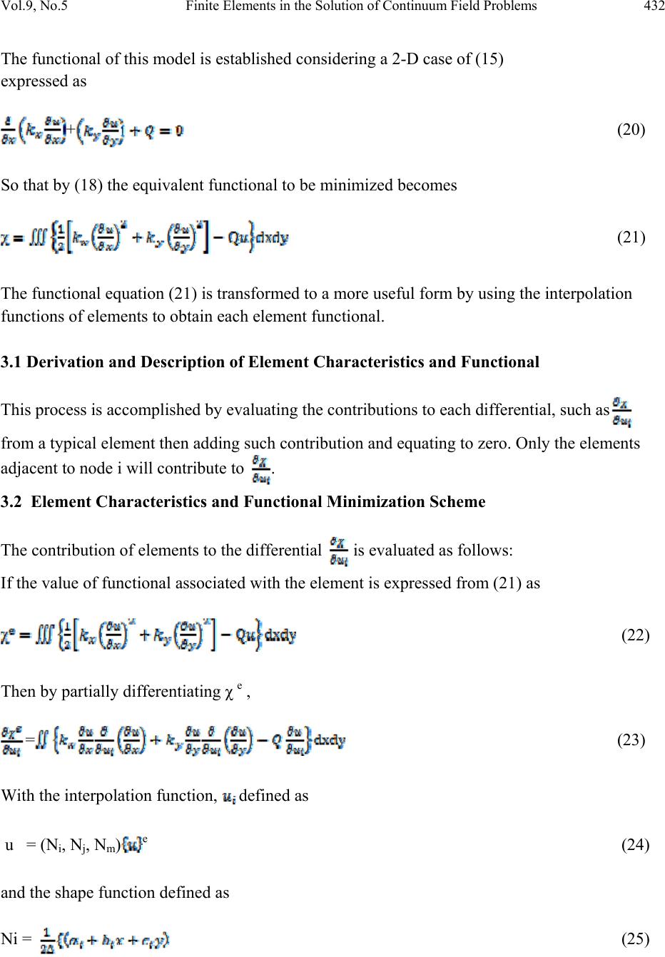 Vol.9, No.5 Finite Elements in the Solution of Continuum Field Problems 432 The functional of this model is established considering a 2-D case of (15) expressed as + (20) So that by (18) the equivalent functional to be minimized becomes (21) The functional equation (21) is transformed to a more useful form by using the interpolation functions of elements to obtain each element functional. 3.1 Derivation and Description of Element Characteristics and Functional This process is accomplished by evaluating the contributions to each differential, such as from a typical element then adding such contribution and equating to zero. Only the elements adjacent to node i will contribute to . 3.2 Element Characteristics and Fun c ti o na l M in im i zation Scheme The contribution of elements to the differential is evaluated as follows: If the value of functional associated with the element is expressed from (21) as (22) Then by partially differentiating χ e , = (23) With the interpolation function, defined as u = (Ni, Nj, Nm)e (24) and the shape function defined as Ni = (25) 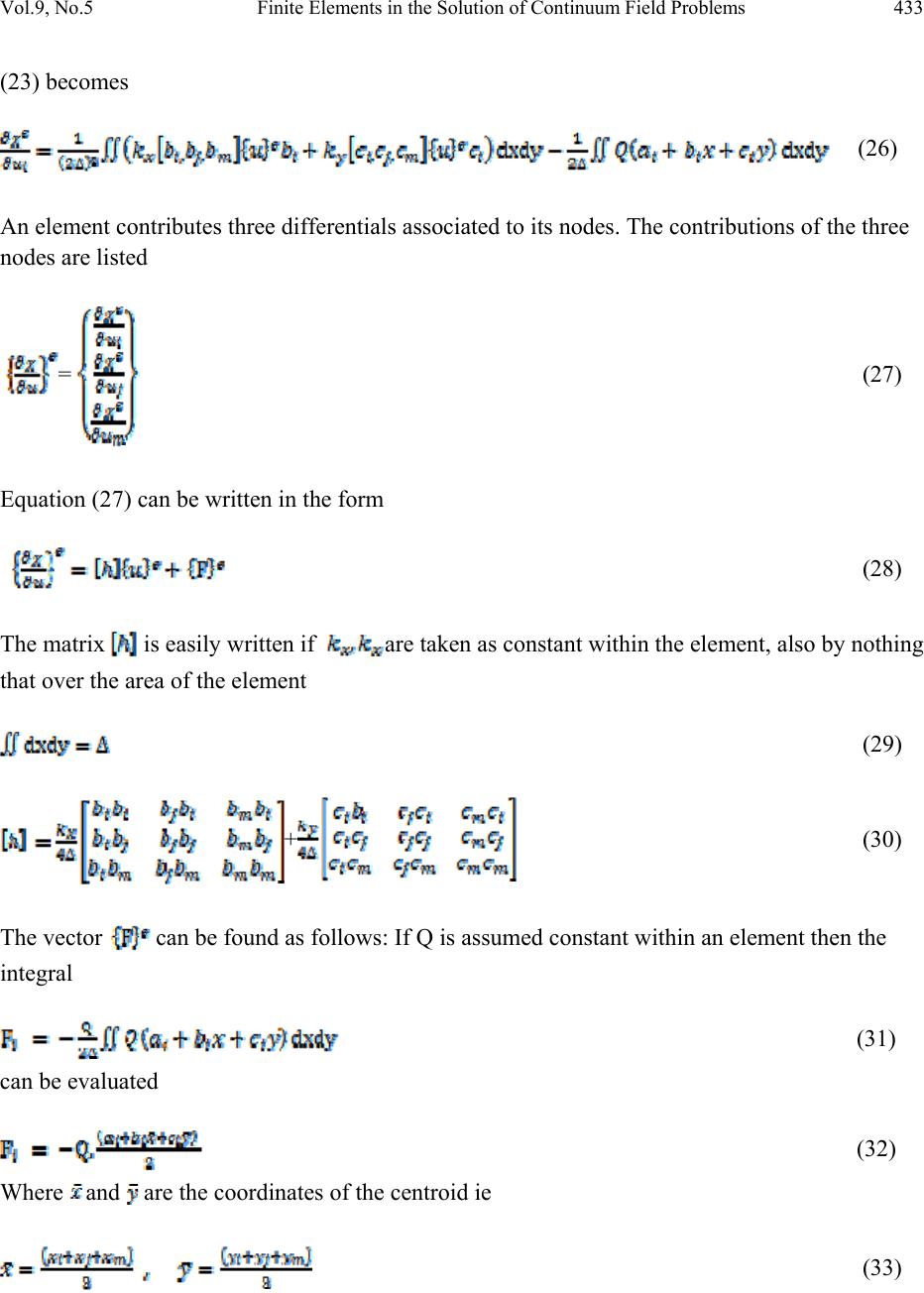 Vol.9, No.5 Finite Elements in the Solution of Continuum Field Problems 433 (23) becomes (26) An element contributes three differentials associated to its nodes. The contributions of the three nodes are listed = (27) Equation (27) can be written in the form (28) The matrix is easily written if are taken as constant within the element, also by nothing that over the area of the element (29) + (30) The vector can be found as follows: If Q is assumed constant within an element then the integral (31) can be evaluated (32) Where and are the coordinates of the centroid ie (33)  Vol.9, No.5 Finite Elements in the Solution of Continuum Field Problems 434 so the integral expressed by (31) becomes (34) 3.3 Assembly Procedure for Functional Minimization Scheme The final equations of the minimization procedure require the assembly of all the differentials of and equating of these to zero, expressed typically as (35) Equation (35) says that the functionals of all elements are established and partially differentiated with respect to the associated nodal degrees of freedoms [11]. 4. METHODOLOGY 4.1 Finite Element Modeling of 2-D Steady State Regional Function Distribution Working in polar coordinates for circular or polar systems in engineering and science often posses some difficulties that this study presents an approximate procedure for processing polar systems as rectangular systems by using the circumference of the circular section as one dimensional independent variable and the difference between the inner and outer radius (thickness) as the second independent variable. The function of interest as the dependent variable is then analysed by solving an approximate function through FEM approaches, which in this study is the Laplace steady state 2-D heat equation in cartesian coordinate. The geometry of field quantities or continuum may be a problem to close form solution of field functions encountered in engineering and science that appropriate algorithm becomes necessary to obtain optimum solution, it is then necessary to employ calculus of variation principles and FEM to obtain optimum continuum field functions whose boundary conditions are specified. In Figure 2, the vertical dimension represents the thickness of a circular pipe or thickness of insulation while the horizontal dimension represents the circumference of circular section of pipe or cylinder. The continuum domain is discretized as shown in Figure 2.  Vol.9, No.5 Finite Elements in the Solution of Continuum Field Problems 435 Figure 2. An Idealized Finite Element Model of a Continuum of GRP Composite . Table 1. Elements Topology Description. Element number Active degrees of freedom for assembly Element coordinates Element nodes 1 u1,u2,u8,v1,v2,v8 (0,0),(17,0),(17,15) 1,2,8 2 U1,u8,u7,v1v8,v7 (0,0),(17,15),(0,15) 1,8,7 3 u2,u3,u7,v2,v3,v7 (17,0),(34,0),(17,15) 2,3,7 4 u2,u7,u8,v2,v7,v8 (17,0),(34,15),(17,15) 2,7,8 5 u3,u4,u10,v3,v4,v10 (34,0),(5,10),(51,15) 3,4,10 6 u3,u10,u9,v3,v10,v9 (34,0),(51,15),(34,15) 3,10,9 7 u4,u5,u11,v4,v5,v11 (51,0),(68,0),(68,15) 4,5,11 8 u4,u11,u10,v4,v111,v10 (51,0),(68,15),(51,15) 4,11,10 9 u5,u6,u12,v5,v6,v12 (68,0),(85,0),(85,15) 5,6,12 10 u5,u12,u11,v5,v12,v11 (68,0),(85,15),(68,15) 5,12,11 11 u7,u8,u14,v7,v8,v14 (0,15),(17,15),(17,30) 7,8,14 123456 131415161718 1 24 3 6 5 8 7 10 9 11 1214 13 16 15 18 17 20 19 127 85mm 30mm y x v u  Vol.9, No.5 Finite Elements in the Solution of Continuum Field Problems 436 12 u7,u14,u13,v7,v14,v13 (0,15),(17,30),(0,30) 7,14,13 13 u8,u9,u15,v8,v9,v15 (17,15),(34,15),(34,30)8,9,15 14 u8,u15,u14,v8,v15,v14 (17,15),(34,30),(17,30)8,15,14 15 u9,u10,u16,v9,v10,v16 (34,15),(51,15),(51,30)9,10.16 16 u9,u16,u15,v9,v16,v15 (34,15),(51,30),(34,30)9,16,15 17 u10,u11,u17,v10,v11,v17 (51,15),(68,15),(68,30)10,11,17 18 u10,u17,u16,v10,v17,v16 (51,15),(68,30),(51,30)10,17,16 19 u11,u12,u18,v11,v12,v18 (68,15),(85,15),(85,30)11,12,18 20 u11,u18,u17,v11,v18,v17 (68,15),(85,30),(68,30)11,18,17 4.2 Computation of Elements Partial Differential Equations By using equation (35) all the systems of partial differential equations are computed for the twenty elements as follows: 4.3 Assumptions The function is assumed to be Laplace function so that equation (28) reduces to (36) and (32) reduces to + (37) By computations of (37) and substitution in (36) for all elements respectively the elements PDEs are presented for twenty elements assembly system as follows: For element 1  Vol.9, No.5 Finite Elements in the Solution of Continuum Field Problems 437 = (38) For element 2 = (39) For element 3 = (40) By application of symmetry the 3by3 matrix in odd numbered elements are equal and similarly for the For element 4 = (41) For element 5 = (42) For element 6 = (43) 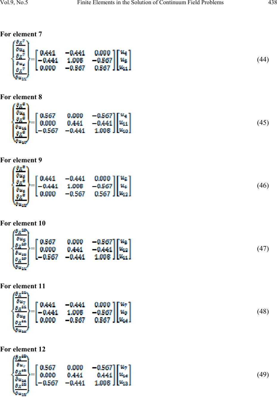 Vol.9, No.5 Finite Elements in the Solution of Continuum Field Problems 438 For element 7 = (44) For element 8 = (45) For element 9 = (46) For element 10 = (47) For element 11 = (48) For element 12 = (49) 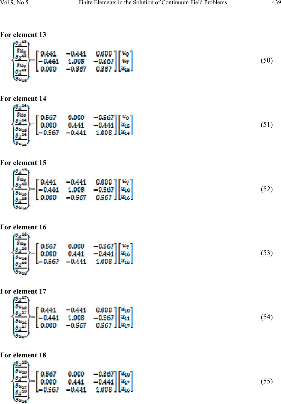 Vol.9, No.5 Finite Elements in the Solution of Continuum Field Problems 439 For element 13 = (50) For element 14 = (51) For element 15 = (52) For element 16 = (53) For element 17 = (54) For element 18 = (55) 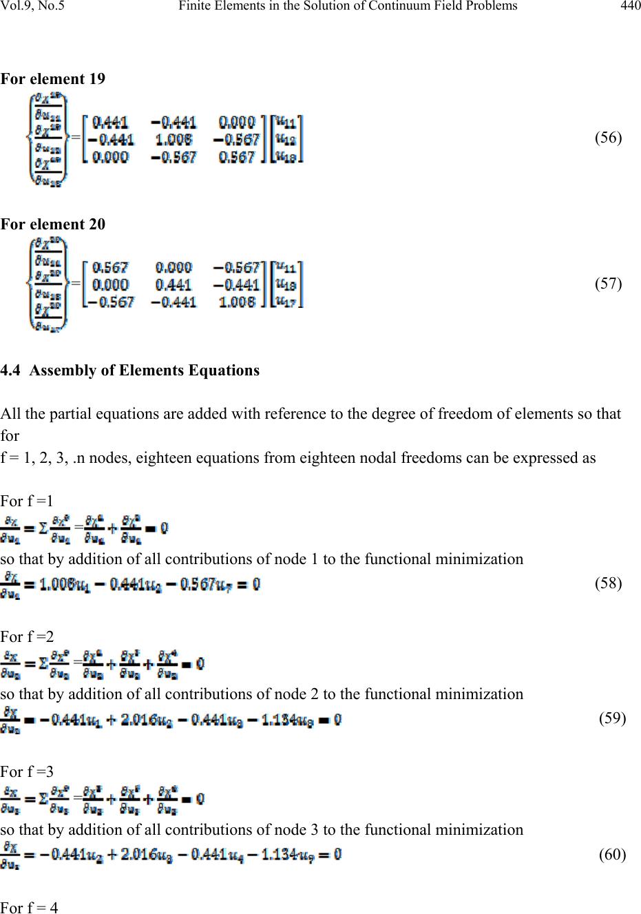 Vol.9, No.5 Finite Elements in the Solution of Continuum Field Problems 440 For element 19 = (56) For element 20 = (57) 4.4 Assembly of Elements Equations All the partial equations are added with reference to the degree of freedom of elements so that for f = 1, 2, 3, .n nodes, eighteen equations from eighteen nodal freedoms can be expressed as For f =1 = so that by addition of all contributions of node 1 to the functional minimization (58) For f =2 = so that by addition of all contributions of node 2 to the functional minimization (59) For f =3 = so that by addition of all contributions of node 3 to the functional minimization (60) For f = 4 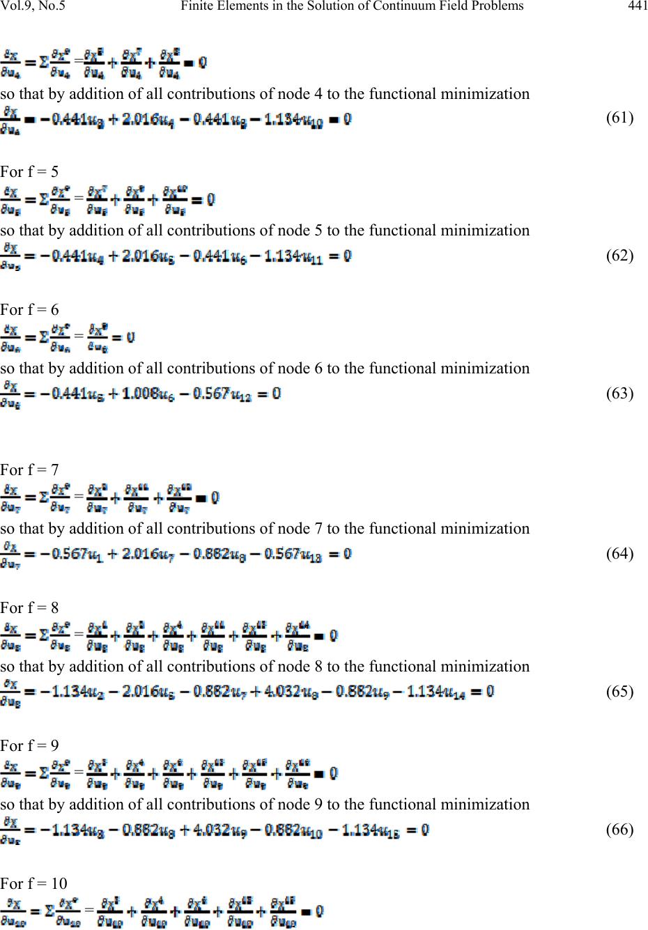 Vol.9, No.5 Finite Elements in the Solution of Continuum Field Problems 441 = so that by addition of all contributions of node 4 to the functional minimization (61) For f = 5 = so that by addition of all contributions of node 5 to the functional minimization (62) For f = 6 = so that by addition of all contributions of node 6 to the functional minimization (63) For f = 7 = so that by addition of all contributions of node 7 to the functional minimization (64) For f = 8 = so that by addition of all contributions of node 8 to the functional minimization (65) For f = 9 = so that by addition of all contributions of node 9 to the functional minimization (66) For f = 10 =  Vol.9, No.5 Finite Elements in the Solution of Continuum Field Problems 442 so that by addition of all contributions of node 10 to the functional minimization (67) For f = 11 = so that by addition of all contributions of node11 to the functional minimization (68) For f = 12 = so that by addition of all contributions of node 12 to the functional minimization (69) For f = 13 = so that by addition of all contributions of node 13 to the functional minimization (70) For f = 14 = so that by addition of all contributions of node 14 to the functional minimization (71) For f = 15 = so that by addition of all contributions of node 15 to the functional minimization (72) For f = 16 = so that by addition of all contributions of node 16 to the functional minimization (73)  Vol.9, No.5 Finite Elements in the Solution of Continuum Field Problems 443 For f = 17 = so that by addition of all contributions of node17 to the functional minimization (74) For f = 18 = so that by addition of all contributions of node 18 to the functional minimization (75) 4.5 Boundary Conditions and Solutions of FEM The above system formed by (58-75) is expressed in FEM matrix format as (76) Where = the vector of the coefficient matrix called the stiffness matrix in FEM terminology = the column vector regarded as the nodal degree of freedom (DOF) = external influence column vector Having established the boundary values of a field function and also the stiffness of the field, the model representing the field response can be solved uniquely. 4.6 Statement of the Field Problem In this study the major objective is to set up FEM that solves continuum functions. To demonstrate the application of this model, thermal field region is solved. The model of (76) is then solved applying the specified boundary conditions of Figure 2: 4.7 Boundary Condition of Hot and Cold Surfaces This may represent the case of a hot fluid in a hollow pipe with outside cold fluid or the case of shell pipe or the case of insulated heat transfer surfaces.  Vol.9, No.5 Finite Elements in the Solution of Continuum Field Problems 444 Figure 3. Schematic Representation of hot and ambient surfaces. By employing (58-75) as (77) (78) (79) (80) (81) (82) and using the boundary conditions as: For ,, the system formed by equation (77-82) reduces to (83) (84) (85) (86) (87) (88) and in matrix form Dimension representing thicknessof pipe Dimension representing thicknessof pipe 123456 1314151617 18 1 24 3 6 5 8 7 10 9 11 1214 13 16 15 18 17 20 19 127 20OC for ambient outside surfaces of a pipe represented by its circumference 50OC for interior hot surfaces of a pipe represented by its circumference  Vol.9, No.5 Finite Elements in the Solution of Continuum Field Problems 445 = (89) (89) is solved by LU-decomposition to obtain , For ,, the system formed by equation (77-82) reduces to = (90) and , For ,, the system formed by equation (77-82) reduces to = (91) and , For ,, the system formed by equation (77-82) reduces to  Vol.9, No.5 Finite Elements in the Solution of Continuum Field Problems 446 = (92) and , For ,, the system formed by equation (77-82) reduces to = (93) and , 5. ANALYSIS OF FEM RESULTS Table 4. Predicted Interior Temperayures Given Boundary Conditions. Ti( oC) Ta( oC) u7(oC) u8(oC) u9(oC) u10(oC) u11(oC) u12(oC) 50 20 47.8089 64.2775 41.7453 36.55796 35.3769 35.1649 50 30 52.8089 69.27747 46.74525 41.55796 40.37687 40.16488 50 40 57.80887 74.27747 51.74525 46.55796 45.37687 45.16488 50 50 62.80889 79.27747 56.74525 51.55796 50.37687 50.16488 50 60 67.80889 84.27747 61.74525 56.5576 55.37687 55.16488 5.1 Regression Modelling of FEM Result The correctness of FEM result is established by using multiple linear regression analysis approach with assumed boundary conditions as dependent variable and FEM predicted interior values of the function as independent variables. This analysis approach enabled the estimation of error associated with FEM and establishment of a design friendly model for the prediction of the 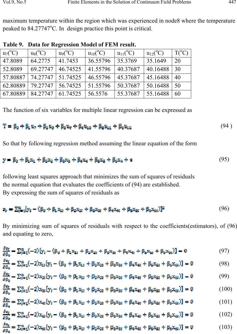 Vol.9, No.5 Finite Elements in the Solution of Continuum Field Problems 447 maximum temperature within the region which was experienced in node8 where the temperature peaked to 84.27747oC. In design practice this point is critical. Table 9. Data for Regression Model of FEM result. u7(oC) u8(oC) u9(oC) u10(oC) u11(oC) u12(oC) T(oC) 47.8089 64.2775 41.7453 36.55796 35.3769 35.1649 20 52.8089 69.27747 46.74525 41.55796 40.37687 40.1648830 57.80887 74.27747 51.74525 46.55796 45.37687 45.1648840 62.80889 79.27747 56.74525 51.55796 50.37687 50.1648850 67.80889 84.27747 61.74525 56.5576 55.37687 55.16488 60 The function of six variables for multiple linear regression can be expressed as (94 ) So that by following regression method assuming the linear equation of the form (95) following least squares approach that minimizes the sum of squares of residuals the normal equation that evaluates the coefficients of (94) are established. By expressing the sum of squares of residuals as (96) By minimizing sum of squares of residuals with respect to the coefficients(estimators), of (96) and equating to zero, (97) (98) (99) (100) (101) (102) (103) 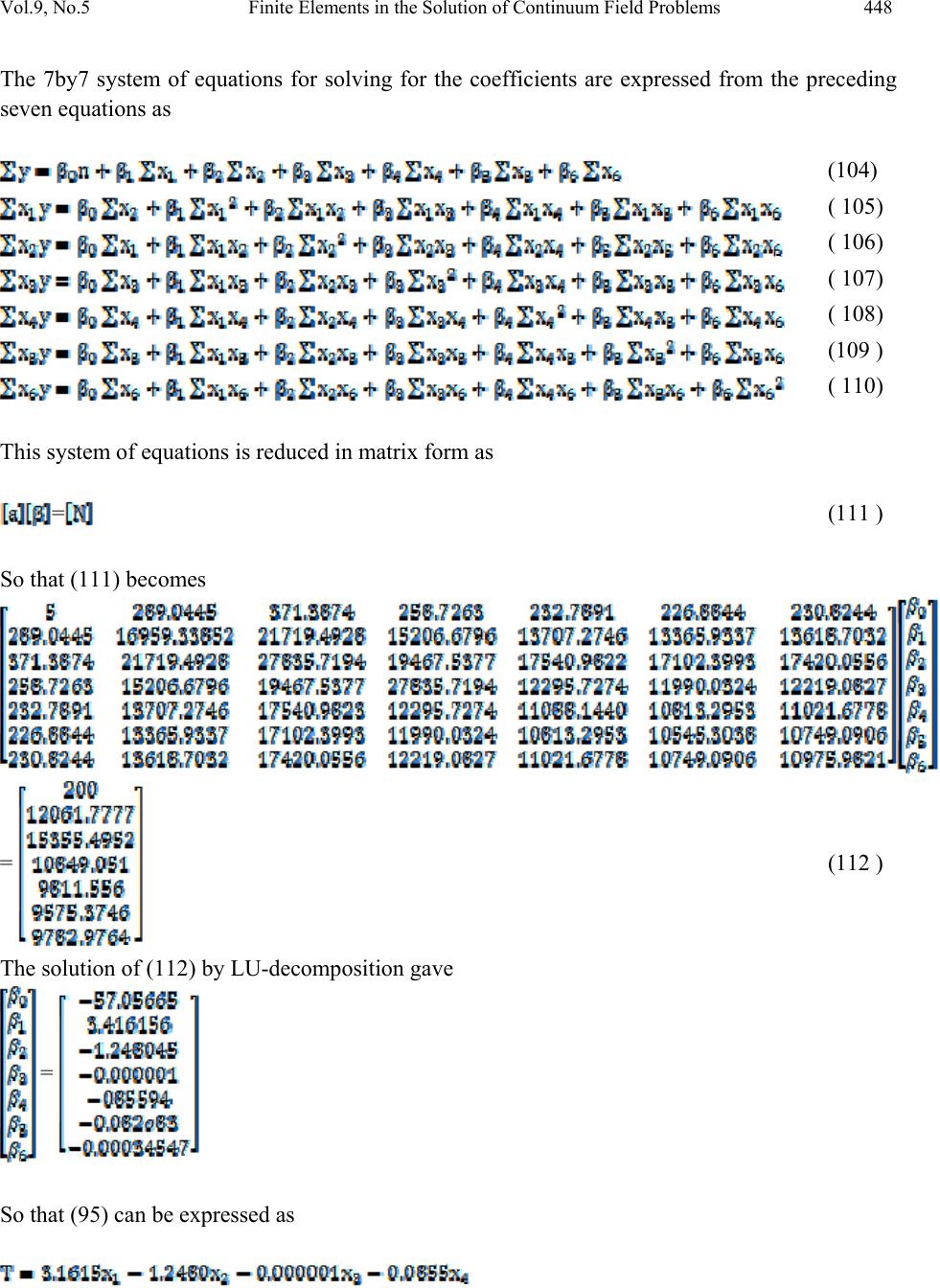 Vol.9, No.5 Finite Elements in the Solution of Continuum Field Problems 448 The 7by7 system of equations for solving for the coefficients are expressed from the preceding seven equations as (104) ( 105) ( 106) ( 107) ( 108) (109 ) ( 110) This system of equations is reduced in matrix form as = (111 ) So that (111) becomes = (112 ) The solution of (112) by LU-decomposition gave = So that (95) can be expressed as 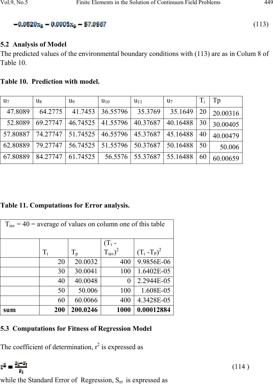 Vol.9, No.5 Finite Elements in the Solution of Continuum Field Problems 449 (113) 5.2 Analysis of Model The predicted values of the environmental boundary conditions with (113) are as in Colum 8 of Table 10. Table 10. Prediction with model. u7 u 8 u 9 u 10 u 11 u 7 T i Tp 47.8089 64.2775 41.7453 36.55796 35.3769 35.16492020.00316 52.8089 69.27747 46.74525 41.55796 40.37687 40.16488 30 30.00405 57.80887 74.27747 51.74525 46.55796 45.37687 45.16488 40 40.00479 62.80889 79.27747 56.74525 51.55796 50.37687 50.16488 5050.006 67.80889 84.27747 61.74525 56.5576 55.37687 55.16488 60 60.00659 Table 11. Computations for Error analysis. Tiav = 40 = average of values on column one of this table Ti T p (Ti - Tiav)2 (Ti -TP)2 20 20.0032 4009.9856E-06 30 30.0041 1001.6402E-05 40 40.0048 02.2944E-05 50 50.006 1001.608E-05 60 60.0066 4004.3428E-05 sum 200 200.0246 10000.00012884 5.3 Computations for Fi tness of Regression Model The coefficient of determination, r2 is expressed as (114 ) while the Standard Error of Regression, Ser is expressed as  Vol.9, No.5 Finite Elements in the Solution of Continuum Field Problems 450 (115) So that by (113 ) and (114) and Table11 6. 3-D PRESENTATION OF RESULTS Table 12. Interior Temperature Distribution at Varyuig Ambient Condition. n 20 oC 30 oC 40oC50 oC60 oC 1 50 50 50 50 50 2 50 50 50 50 50 3 50 50 50 50 50 4 50 50 50 50 50 5 50 50 50 50 50 6 50 50 50 50 50 7 47.8089 52.8089 57.8088762.8088967.80889 8 64.2775 69.27747 74.2774779.2774784.27747 9 41.7453 46.74525 45.3768756.7452561.74525 10 36.55796 41.55796 45.16488 51.55796 56.5576 11 35.3769 40.37687 35.3768 50.3768755.37687 12 35.169 40.16488 35.1649 50.1648855.16488 13 20 30 40 50 60 14 20 30 40 50 60 15 20 30 40 50 60 16 20 30 40 50 60 17 20 30 40 50 60 18 20 30 40 50 60  Vol.9, No.5 Finite Elements in the Solution of Continuum Field Problems 451 Figure 4. Line plot to depiction of temperature at nodal points using Table 12. Figure 5. 3-D plot of temperature at nodal points using Table 10. 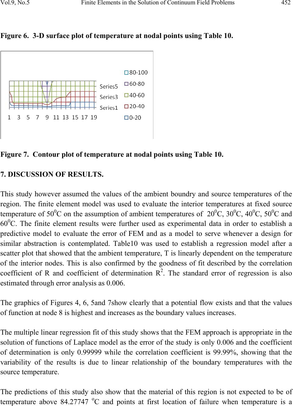 Vol.9, No.5 Finite Elements in the Solution of Continuum Field Problems 452 Figure 6. 3-D surface plot of temperature at nodal points using Table 10. Figure 7. Contour plot of temperature at nodal points using Table 10. 7. DISCUSSION OF RESULTS. This study however assumed the values of the ambient boundry and source temperatures of the region. The finite element model was used to evaluate the interior temperatures at fixed source temperature of 500C on the assumption of ambient temperatures of 200C, 300C, 400C, 500C and 600C. The finite element results were further used as experimental data in order to establish a predictive model to evaluate the error of FEM and as a model to serve whenever a design for similar abstraction is contemplated. Table10 was used to establish a regression model after a scatter plot that showed that the ambient temperature, T is linearly dependent on the temperature of the interior nodes. This is also confirmed by the goodness of fit described by the correlation coefficient of R and coefficient of determination R2. The standard error of regression is also estimated through error analysis as 0.006. The graphics of Figures 4, 6, 5and 7show clearly that a potential flow exists and that the values of function at node 8 is highest and increases as the boundary values increases. The multiple linear regression fit of this study shows that the FEM approach is appropriate in the solution of functions of Laplace model as the error of the study is only 0.006 and the coefficient of determination is only 0.99999 while the correlation coefficient is 99.99%, showing that the variability of the results is due to linear relationship of the boundary temperatures with the source temperature. The predictions of this study also show that the material of this region is not expected to be of temperature above 84.27747 oC and points at first location of failure when temperature is a  Vol.9, No.5 Finite Elements in the Solution of Continuum Field Problems 453 critical design parameter. The quantity of heat attained by the material of this study can be quantified by the predictions of this study when appropriate relations are applied. 8. CONCLUSSIONS The procedure of this study presented the basis for insulation design for solid, hollow or shell pipes in fluid transport design in oil and gas transport system. The finite element method evaluated the temperature distribution of the region to serve as a guide to quantify heat to the environment from the transit fluid. This study also presents an approximate procedure for processing polar systems as rectangular systems by using the circumference of the circular section as one dimensional independent variable and the difference between the inner and outer radius (thickness) as the second independent variable. Above all the multiple linear regression fit of predictions of this study shows that the FEM approach is appropriate in the solution of functions of Laplace model as the error of the study is only 0.006 and the coefficient of determination is only 0.99999 while the correlation coefficient is 0.99999(99.99%), showing that the boundary temperature is linearly related to the interior or the source temperature. The predictions of this study also show that the material of this region is not expected to be of temperature above 84.27747oC and that the quantity of heat attained by the material of this study can be quantified when appropriate relations are applied. REFERENCES [1] Sundaram,V., Balasubramanian, R., Lakshminarayanan,K.A.,(2003) Engineering Mathematics ,Vol.3,VIKAS Publishing House LTD, New Delhi, p173. [2] Holman, J. P, (1981) Heat and mass Transfer, McGraw-Hill Inc.Book Company, p72. [3] Cook,R.D., Malkus, D.S. and Plesha,M.E.(1989) Concepts and Applications of Finite Element Analysis, 3 rd ed, John Wiley & Sons, New York in Astley, R.J., (1992), Finite Elements in Solids and Structures, Chapman and Hall Publishers, UK, p77. [4] Bathe, K.J., and Wilson, E.L. (1976) Numerical Methods in Finite Element Analysis, Prentice Hall, Englewood Cliffs. [5] Hughes,T.J.R. (1987) The Finite Element Method : Linear Static and Dynamic Finite Element Analysis, Prentice hall, Englewood Cliffs, . [6] Enetanya A. N. and Ihueze C. C., (2009) Finite Difference Approach for Optimum Compressive Strengths of GRP Composites, NSE TECHNICAL TRANSACTIONS,July.September, 2009,Vol.44 No3,p 40-55 [7] Astley, R.J., (1992), Finite Elements in Solids and Structures, Chapman and Hall Publishers,UK, p77.  Vol.9, No.5 Finite Elements in the Solution of Continuum Field Problems 454 [8] Zienkiewicz,O.C., and Cheung, Y.K,(1967) The Finite Element in Structural and Continuum Mechanics, McGraw-Hill publishing Coy Ltd, London, p148 [9] Amazigo, J.C and Rubenfield, L.A (1980) Advanced Calculus and its application to the Engineering and Physical Sciences, John Wiley and sons Publishing, New York, p130. [10] Berg P. N (1962 ) Calculus of variations, in Handbook of Engineering Mechanics, chapter 16, ed. W. Flugge, Graw-Hill. [11] Ihueze, C. C,Umenwaliri,S.Nand Dara,J.E (2009) Finite Element Approach to Solution of Multidimensional Field Functions, African Research Review: An International Multi- Disciplinary Journal, Vol.3(5),October,2009, Ethiopia,p437-457. |