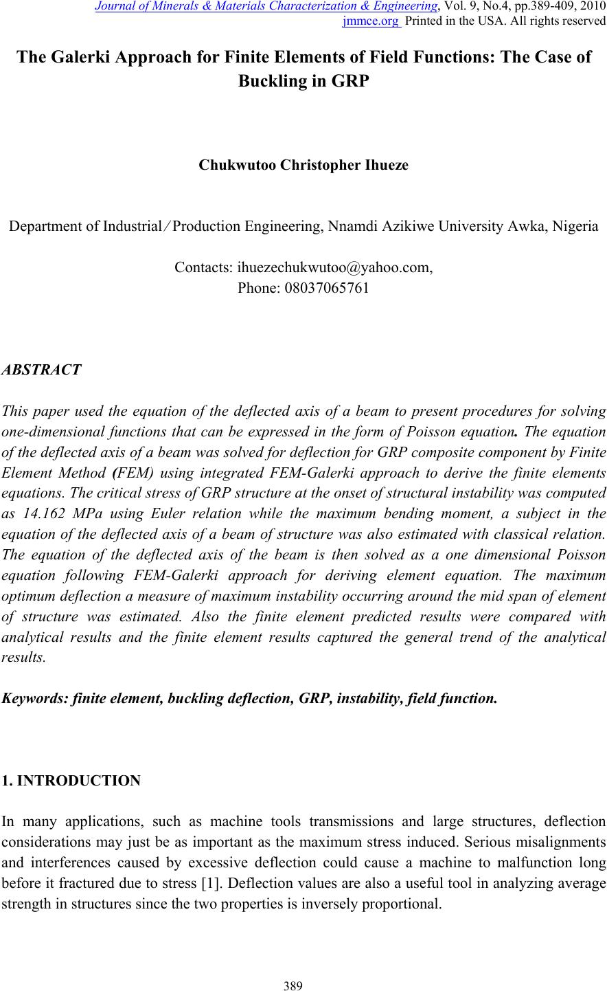Journal of Minerals & Materials Characterization & Engineering, Vol. 9, No.4, pp.389-409, 2010
jmmce.org Printed in the USA. All rights reserved
389
The Galerki Approach for Finite E l e m e n ts o f F i el d Functions: The Case of
Buckling in G R P
Chukwutoo Christopher Ihueze
Department of Industrial ⁄ Production Engineering, Nnamdi Azikiwe University Awka, Nigeria
Contacts: [e-mail],
Phone: [phone]
ABSTRACT
This paper used the equation of the deflected axis of a beam to present procedures for solving
one-dimensional functions that can be expressed in the form of Poisson equation. The equation
of the deflected axis of a beam was solved for deflection for GRP composite component by Finite
Element Method (FEM) using integrated FEM-Galerki approach to derive the finite elements
equations. The critical stress of GRP structure at the onset of structural instability was computed
as 14.162 MPa using Euler relation while the maximum bending moment, a subject in the
equation of the deflected axis of a beam of structure was also estimated with classical relation.
The equation of the deflected axis of the beam is then solved as a one dimensional Poisson
equation following FEM-Galerki approach for deriving element equation. The maximum
optimum deflection a measure of maximum instability occurring aro und the mid span of element
of structure was estimated. Also the finite element predicted results were compared with
analytical results and the finite element results captured the general trend of the analytical
results.
Keywords: finite element, buckling deflection, GRP, instability, field function.
1. INTRODUCTION
In many applications, such as machine tools transmissions and large structures, deflection
considerations may just be as important as the maximum stress induced. Serious misalignments
and interferences caused by excessive deflection could cause a machine to malfunction long
before it fractured due to stress [1]. Deflection values are also a useful tool in analyzing average
strength in structures since the two properties is inversely proportional.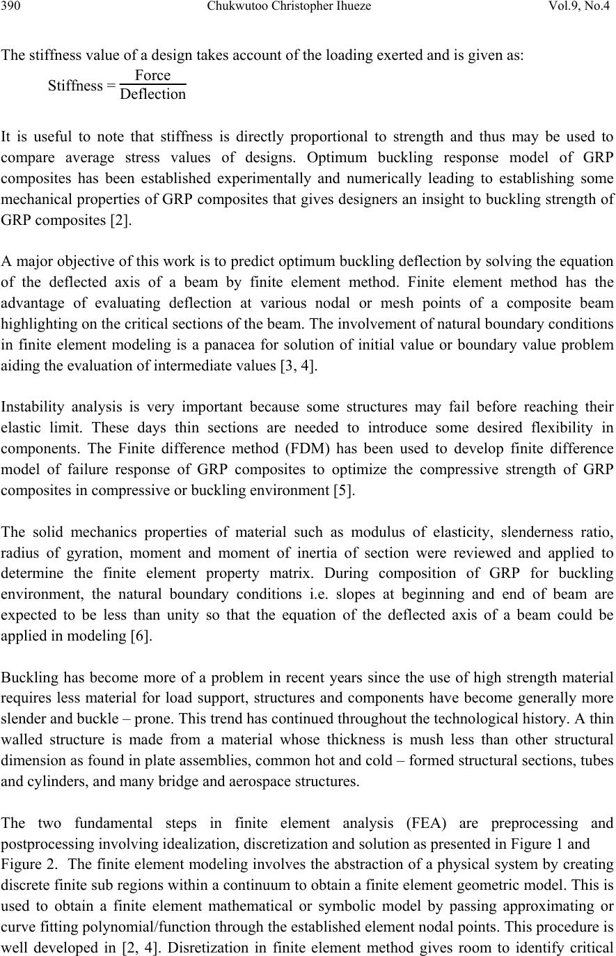

390 Chukwutoo Christopher Ihueze Vol.9, No.4
The stiffness value of a design takes account of the loading exerted and is given as:
Stiffness =
Force
Deflection
It is useful to note that stiffness is directly proportional to strength and thus may be used to
compare average stress values of designs. Optimum buckling response model of GRP
composites has been established experimentally and numerically leading to establishing some
mechanical properties of GRP composites that gives designers an insight to buckling strength of
GRP composites [2].
A major objective of this work is to predict optimum buckling deflection by solving the equation
of the deflected axis of a beam by finite element method. Finite element method has the
advantage of evaluating deflection at various nodal or mesh points of a composite beam
highlighting on the critical sections of the beam. The involvement of natural boundary conditions
in finite element modeling is a panacea for solution of initial value or boundary value problem
aiding the evaluation of intermediate values [3, 4].
Instability analysis is very important because some structures may fail before reaching their
elastic limit. These days thin sections are needed to introduce some desired flexibility in
components. The Finite difference method (FDM) has been used to develop finite difference
model of failure response of GRP composites to optimize the compressive strength of GRP
composites in compressive or buckling environment [5].
The solid mechanics properties of material such as modulus of elasticity, slenderness ratio,
radius of gyration, moment and moment of inertia of section were reviewed and applied to
determine the finite element property matrix. During composition of GRP for buckling
environment, the natural boundary conditions i.e. slopes at beginning and end of beam are
expected to be less than unity so that the equation of the deflected axis of a beam could be
applied in modeling [6].
Buckling has become more of a problem in recent years since the use of high strength material
requires less material for load support, structures and components have become generally more
slender and buckle – prone. This trend has continued throughout the technological history. A thin
walled structure is made from a material whose thickness is mush less than other structural
dimension as found in plate assemblies, common hot and cold – formed structural sections, tubes
and cylinders, and many bridge and aerospace structures.
The two fundamental steps in finite element analysis (FEA) are preprocessing and
postprocessing involving idealization, discretization and solution as presented in Figure 1 and
Figure 2. The finite element modeling involves the abstraction of a physical system by creating
discrete finite sub regions within a continuum to obtain a finite element geometric model. This is
used to obtain a finite element mathematical or symbolic model by passing approximating or
curve fitting polynomial/function through the established element nodal points. This procedure is
well developed in [2, 4]. Disretization in finite element method gives room to identify critical

Vol.9, No.4 The Galerki Approach for Finite Elements of Field Functions 391
location for point of first failure. Composites in general have random material properties as many
materials are involved as constituents during the formative stage.
2. THEORETICAL BACKGROUND ON COMPRESSIVE FAILURE OF BEAM.
A horizontal beam situated on the x axis of an xy coordinate system and supported at both ends
bends under the influence of axial compressive loads as depicted in Figure 1. The deflection
curve of the beam often called the elastic curve is also shown in Figure 1
Figure 1. Beam compressive loading and deflected beam axis.
Following Figure 1, Euler 1774 expressed the minimum buckling model of engineering member
subjected to axial compression within its materials elastic limit provided that the greatest
dimension is more than 4 to 6 times its least cross sectional size as
P =
Π2EJ
L (1)
The buckling stress, critical stress, following equation (1) is classically expressed as
Sc =
Π2E
∧2 (2)
Equation (1) was derived by employing the well known equation of deflected axis of a beam
usually expressed as
EJ ∂2y
∂x2 = M(x) (3)
The maximum compressive stress of a beam subject to axial compression is expressed in [6] as
S = P
A +Mc J (4)
where
E = modulus of elasticity of material
L
y
y
P x
P

392 Chukwutoo Christopher Ihueze Vol.9, No.4
J = moment of inertia of section
A = area of cross section
c = dimension representing the position of neutral axis of section
P = critical load
L= length of section
Sc = critical stress
The critical stress of beam under compressive loading is expressed in [7].
Equation (4) shows that when a beam is subjected to axial compression, stress due to axial load
and stress due to induced moment are set up. The computing model for moment of inertia and
slenderness ratio of section is expressed in [8] as
J = Ak2 = bd3
3 = b √3 (5)
and
∧ = L
k , c = depth of section 2 (6)
where
∧ = slenderness ratio.
k = radius of gyration of section.
b = breath of section
d = depth of section.
The maximum compressive strength of GRP composites is 50% its tensile strength [9, 10, 11].
Also reported in [9] is that the tensile strength of GRP composite is about 303 MPa so that the
compressive strength becomes about 152 MPa. Equation (4) could then be re-expressed as
152 =
P
A +Mc J (7)
Equation (7) shows that as bending of member decreases the compressive strength becomes due
to axial compression alone so that the maximum compressive strength becomes due to axial
compression. Equation (4) becomes, by using the result of [2] by [5] and assumption of [9],
154 =
P
A ± Mc J (8)
From Euler 1774, the critical force Pc = P, so that
P
A = Pc A = Π2E
∧2 (9)

Vol.9, No.4 The Galerki Approach for Finite Elements of Field Functions 393
Equation (8) may be re-expressed as
154 =
Π2E
∧2 ± Mc
J (10)
The basic properties of materials of structure like modulus of elasticity and moment of inertia of
section are found by employing the equation of deflected axis of a beam with some
experimentally derived data expressed as
EJ ∂2y
∂x2 = M(x)
so that by subject of formula
∂2y
∂x2 = M(x) EJ (11)
By method of weighted residual, equation (11) becomes
R = ∂2y
∂x2 - M(x) EJ (12)
3. METHODOLOGY
Finite elements formulation involves discretizing, choice of approximating polynomial,
derivation of shape function, interpolation functions, and expression of element equations in
terms of interpolation functions. The basic steps of FEM are found in [4, 12]. The Galerki
method was used in deriving element and assembly equations while LU-decomposition is used in
obtaining solutions. The basic steps used with Galerki method to obtain the finite element results
involve:
• Discretization
• Proposing polynomial interpolation within the element, the number of unknown
coefficients being equal to the number of nodes defining the topology of the
element
• Evaluation of interpolation at each node and equating to the nodal displacement.
This gives a set of simultaneous linear equations which will be solved to yield the
unknown polynomial coefficients.
• Substitution of expression of coefficients into the original interpolation
(approximation polynomial) and the arrangement of terms to yield an expression
of the form(shape function)
u(x) = N1(x)y1 + N2(x)y2 +.................... (13)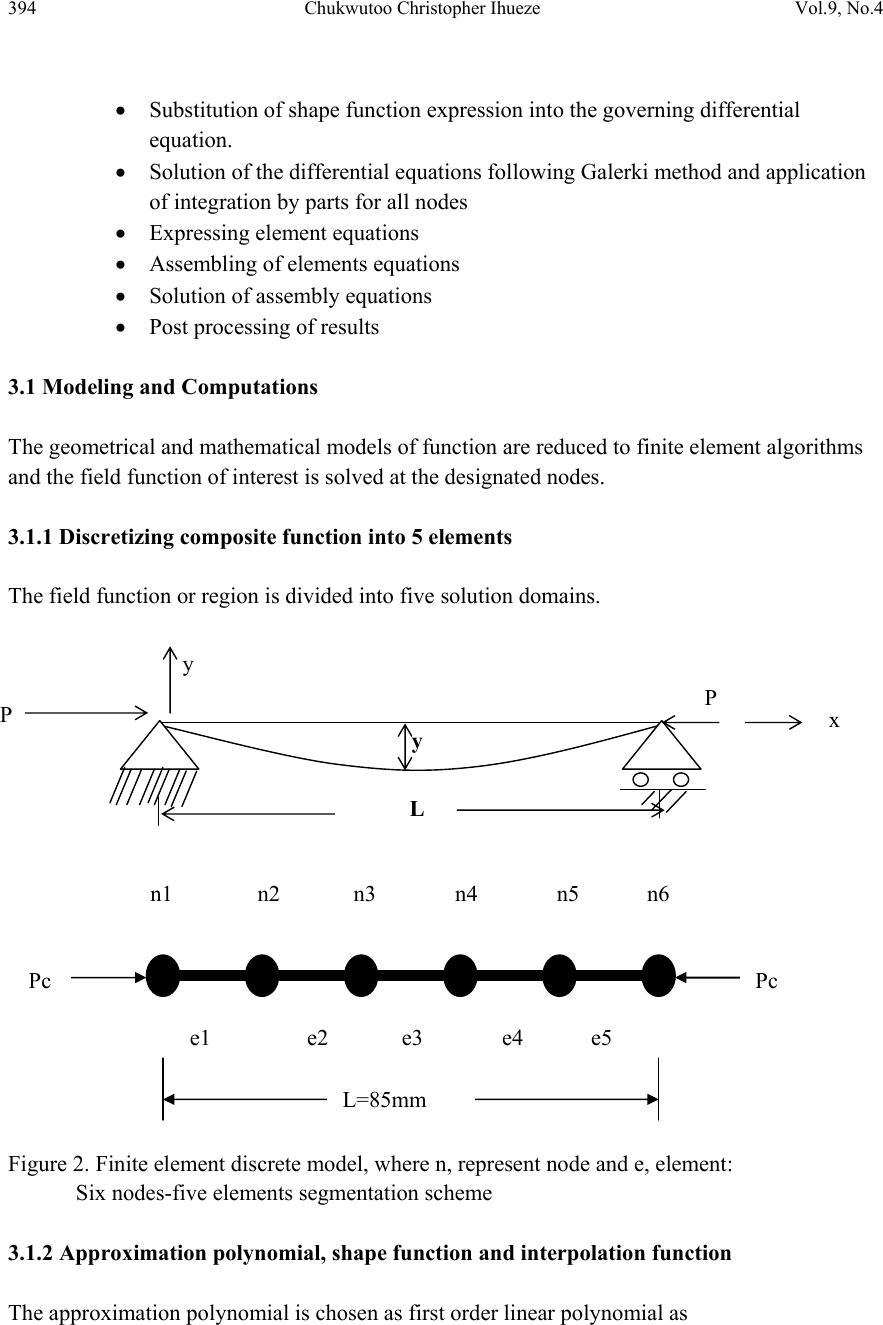

394 Chukwutoo Christopher Ihueze Vol.9, No.4
• Substitution of shape function expression into the governing differential
equation.
• Solution of the differential equations following Galerki method and application
of integration by parts for all nodes
• Expressing element equations
• Assembling of elements equations
• Solution of assembly equations
• Post processing of results
3.1 Modeling and Computations
The geometrical and mathematical models of function are reduced to finite element algorithms
and the field function of interest is solved at the designated nodes.
3.1.1 Discretizing composite function into 5 elements
The field function or region is divided into five solution domains.
Figure 2. Finite element discrete model, where n, represent node and e, element:
Six nodes-five elements segmentation scheme
3.1.2 Approximation polynomial, shape function and interpolation function
The approximation polynomial is chosen as first order linear polynomial as
Pc Pc
L=85mm
n1 n2 n3 n4 n5 n6
e1 e2 e3 e4 e5
L
y
y
P x
P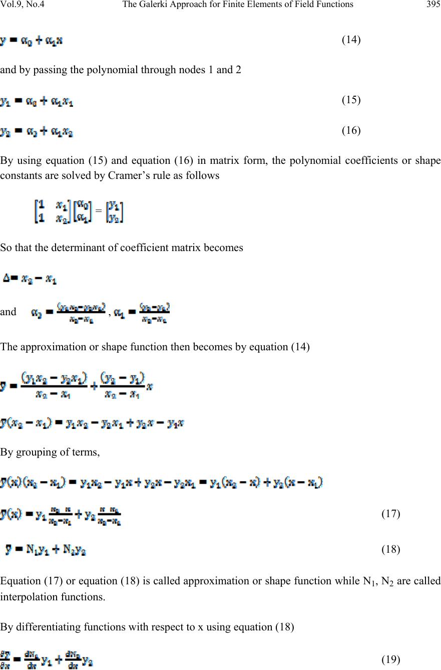

Vol.9, No.4 The Galerki Approach for Finite Elements of Field Functions 395
(14)
and by passing the polynomial through nodes 1 and 2
(15)
(16)
By using equation (15) and equation (16) in matrix form, the polynomial coefficients or shape
constants are solved by Cramer’s rule as follows
=
So that the determinant of coefficient matrix becomes
and ,
The approximation or shape function then becomes by equation (14)
By grouping of terms,
(17)
(18)
Equation (17) or equation (18) is called approximation or shape function while N1, N2 are called
interpolation functions.
By differentiating functions with respect to x using equation (18)
(19)

396 Chukwutoo Christopher Ihueze Vol.9, No.4
From (4)
(20)
(21)
3.2 Galerki Method for Eelement Equation: The Method of Weighted Residuals (MWR)
By employing the equation of a deflected axis of a beam as
(22)
By passing equation (18) through equation (22),
(23)
Since equation (18) does not give the exact value of the function, equation (23) can be expressed
as
(24)
MWR suggests that
(24a)
Wi = linearly independent weighting functions
By finite element procedure, Wi = Ni so that equation (24a) becomes
(25)
By using equation (15) in the Galerki method equation of equation (25), the one dimensional
compression equation of equation (22) becomes
(26)

Vol.9, No.4 The Galerki Approach for Finite Elements of Field Functions 397
Equation (26) can be expressed as
(27)
Integration by parts is used to simplify the L.H.S of equation (27)
(28)
so that by Choosing
(29)
By evaluating the terms in equation (29)
For i = 1
(30)
For i = 2
(31)
Substituting equation (30) and equation (31) in equation (29) and then in equation (27),
For i = 1
(32)
For i = 2
(33)
But x1 = 0, x2 = 17
By evaluating equation (32) and equation (33) the element 1 equations are established.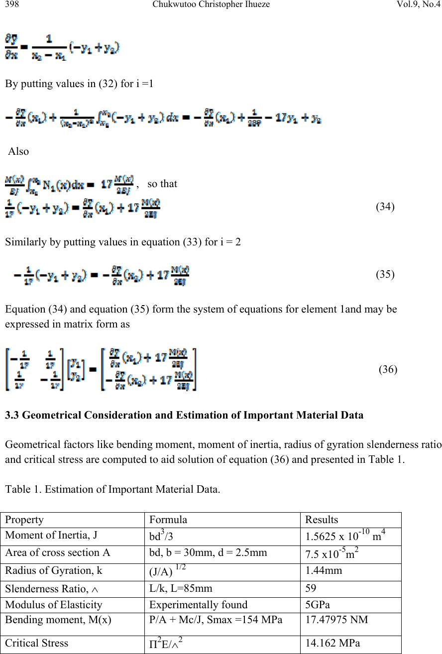

398 Chukwutoo Christopher Ihueze Vol.9, No.4
By putting values in (32) for i =1
Also
, so that
(34)
Similarly by putting values in equation (33) for i = 2
(35)
Equation (34) and equation (35) form the system of equations for element 1and may be
expressed in matrix form as
(36)
3.3 Geometrical Consideration and Estimation of Important Material Data
Geometrical factors like bending moment, moment of inertia, radius of gyration slenderness ratio
and critical stress are computed to aid solution of equation (36) and presented in Table 1.
Table 1. Estimation of Important Material Data.
Property Formula Results
Moment of Inertia, J bd3/3 1.5625 x 10-10 m4
Area of cross section A bd, b = 30mm, d = 2.5mm 7.5 x10-5m2
Radius of Gyration, k (J/A) 1/2 1.44mm
Slenderness Ratio, ∧ L/k, L=85mm 59
Modulus of Elasticity Experimentally found 5GPa
Bending moment, M(x) P/A + Mc/J, Smax =154 MPa 17.47975 NM
Critical Stress Π2E/∧2 14.162 MPa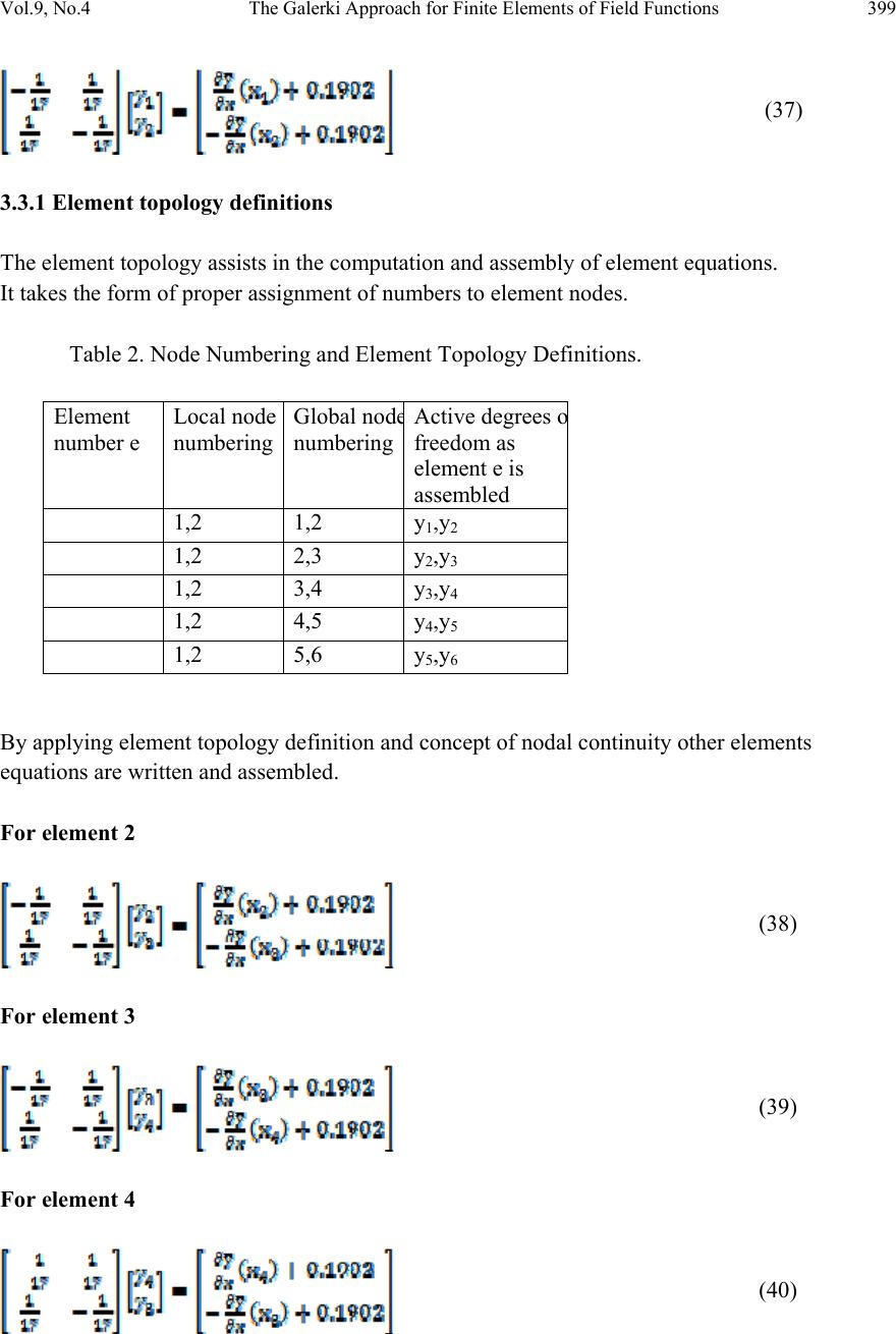

Vol.9, No.4 The Galerki Approach for Finite Elements of Field Functions 399
(37)
3.3.1 Element topology definitions
The element topology assists in the computation and assembly of element equations.
It takes the form of proper assignment of numbers to element nodes.
Table 2. Node Numbering and Element Topology Definitions.
By applying element topology definition and concept of nodal continuity other elements
equations are written and assembled.
For element 2
(38)
For element 3
(39)
For element 4
(40)
Element
number e
Local node
numbering
Global nod
e
numbering
Active degrees
o
freedom as
element e is
assembled
1,2 1,2 y1,y2
1,2 2,3 y2,y3
1,2 3,4 y3,y4
1,2 4,5 y4,y5
1,2 5,6 y5,y6

400 Chukwutoo Christopher Ihueze Vol.9, No.4
For element 5
(41)
Where
y
1
= Active degree of freedom representing deflection at node 1
y
2 = Active degree of freedom representing deflection at node 2
y
3 = Active degree of freedom representing deflection at node 3
y
4 = Active degree of freedom representing deflection at node 4
y
5 = Active degree of freedom representing deflection at node 5
y
6 = Active degree of freedom representing deflection at node 6
x
1 = first nodal position
x
2 = second nodal position
x
3 = third nodal position
x
4 = fourth nodal position
x
5 = fifth nodal position
x
6 = sixth nodal position
3.4 Assembling and Derivation of Elements Assembly Equation
The respective element equations are established from elements topology descriptions and are
added randomly into the initialized assembly matrices describing the property matrix, boundary
influence matrix and external effects matrix as follows. The assembling is done element
equations after element equations with respect to elements degrees of freedom or variables
present in the element equations, until the final element equation is assembled to obtain the
assembly equation as in equation (43)
3.4.1 Initialized assembly zero matrix
The initial matrix to aid assembly of elements matrixes can be expressed as
= (42)
By random addition of matrixes of equations ((37) - (41)) into equation (42) the assembly
equation is obtained after all the 2x2 element matrixes of equations ((37) - (41)) are transformed
to 6 x 6 matrixes.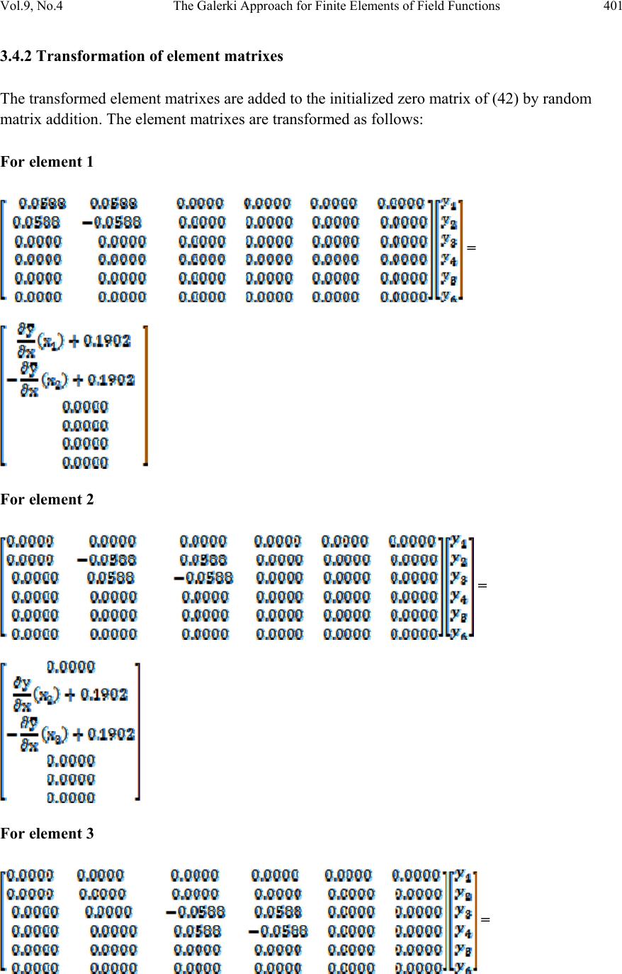

Vol.9, No.4 The Galerki Approach for Finite Elements of Field Functions 401
3.4.2 Transformation of element matrixes
The transformed element matrixes are added to the initialized zero matrix of (42) by random
matrix addition. The element matrixes are transformed as follows:
For element 1
=
For element 2
=
For element 3
=

402 Chukwutoo Christopher Ihueze Vol.9, No.4
For element 4
=
For element 5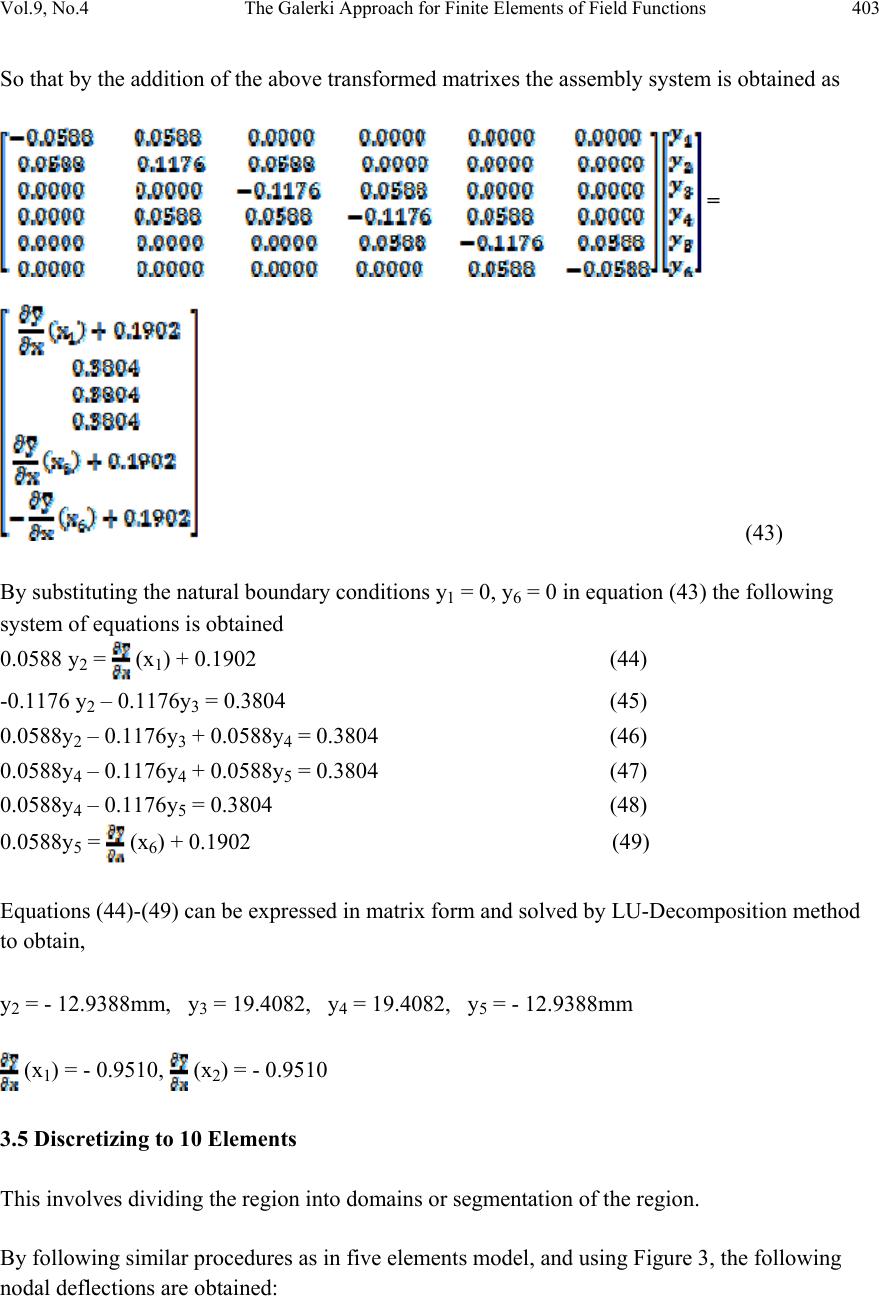
=

Vol.9, No.4 The Galerki Approach for Finite Elements of Field Functions 403
So that by the addition of the above transformed matrixes the assembly system is obtained as
=
(43)
By substituting the natural boundary conditions y1 = 0, y6 = 0 in equation (43) the following
system of equations is obtained
0.0588 y2 = (x1) + 0.1902 (44)
-0.1176 y2 – 0.1176y3 = 0.3804 (45)
0.0588y2 – 0.1176y3 + 0.0588y4 = 0.3804 (46)
0.0588y4 – 0.1176y4 + 0.0588y5 = 0.3804 (47)
0.0588y4 – 0.1176y5 = 0.3804 (48)
0.0588y5 = (x6) + 0.1902 (49)
Equations (44)-(49) can be expressed in matrix form and solved by LU-Decomposition method
to obtain,
y2 = - 12.9388mm, y3 = 19.4082, y4 = 19.4082, y5 = - 12.9388mm
(x1) = - 0.9510, (x2) = - 0.9510
3.5 Discretizing to 10 Elements
This involves dividing the region into domains or segmentation of the region.
By following similar procedures as in five elements model, and using Figure 3, the following
nodal deflections are obtained: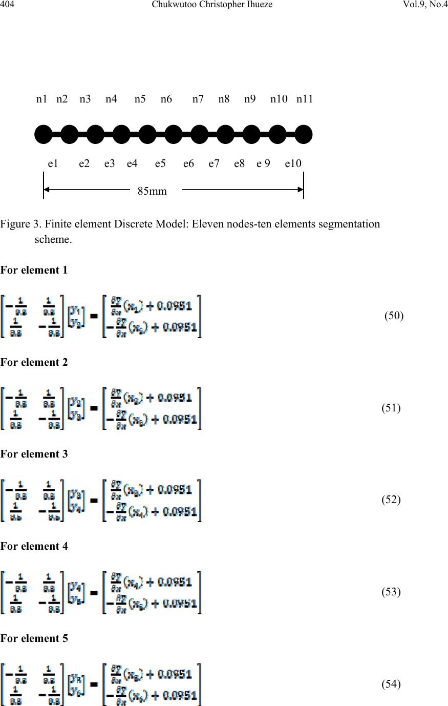

404 Chukwutoo Christopher Ihueze Vol.9, No.4
Figure 3. Finite element Discrete Model: Eleven nodes-ten elements segmentation
scheme.
For element 1
(50)
For element 2
(51)
For element 3
(52)
For element 4
(53)
For element 5
(54)
85mm
n1 n2 n
3
n4 n
5
n
6
n
7
n
8
n
9
n1
0
n11
e
1
e
2
e3
e
4
e5
e6
e7
e8
e
9
e
1
0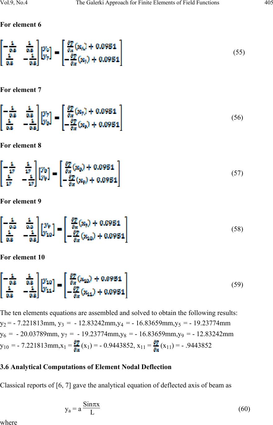

Vol.9, No.4 The Galerki Approach for Finite Elements of Field Functions 405
For element 6
(55)
For element 7
(56)
For element 8
(57)
For element 9
(58)
For element 10
(59)
The ten elements equations are assembled and solved to obtain the following results:
y2 = - 7.221813mm, y3 = - 12.83242mm,y4 = - 16.83659mm,y5 = - 19.23774mm
y6 = - 20.03789mm, y7 = - 19.23774mm,y8 = - 16.83659mm,y9 = - 12.83242mm
y10 = - 7.221813mm,x1 = (x1) = - 0.9443852, x11 = (x11) = - .9443852
3.6 Analytical Computations of Element Nodal Deflection
Classical reports of [6, 7] gave the analytical equation of deflected axis of beam as
ya = a Sinπx
L (60)
where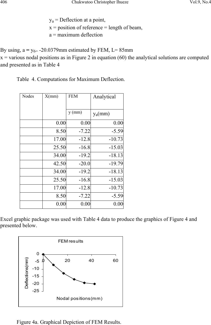

406 Chukwutoo Christopher Ihueze Vol.9, No.4
ya = Deflection at a point,
x = position of reference = length of beam,
a = maximum deflection
By using, a = y6= -20.0379mm estimated by FEM, L= 85mm
x = various nodal positions as in Figure 2 in equation (60) the analytical solutions are computed
and presented as in Table 4
Table 4. Computations for Maximum Deflection.
Excel graphic package was used with Table 4 data to produce the graphics of Figure 4 and
presented below.
FEM results
-25
-20
-15
-10
-5
0
0204060
Nodal posit ions(mm)
Defl ections(mm)
Figure 4a. Graphical Depiction of FEM Results.
Nodes X(mm) FEM Analytical
y (mm) ya(mm)
0.00
0
0.00
0
0.00
0
8.50
0
-7.22 -5.59
0
17.00
0
-12.8
3
-10.73
7
25.50
0
-16.8
3
-15.03
34.00
0
-19.2
3
-18.13
42.50
0
-20.0
3
-19.79
34.00
0
-19.2
3
-18.13
25.50
0
-16.8
3
-15.03
17.00
0
-12.8
3
-10.73
7
8.50
0
-7.22 -5.59
0
0.00
0
0.00
0
0.00
0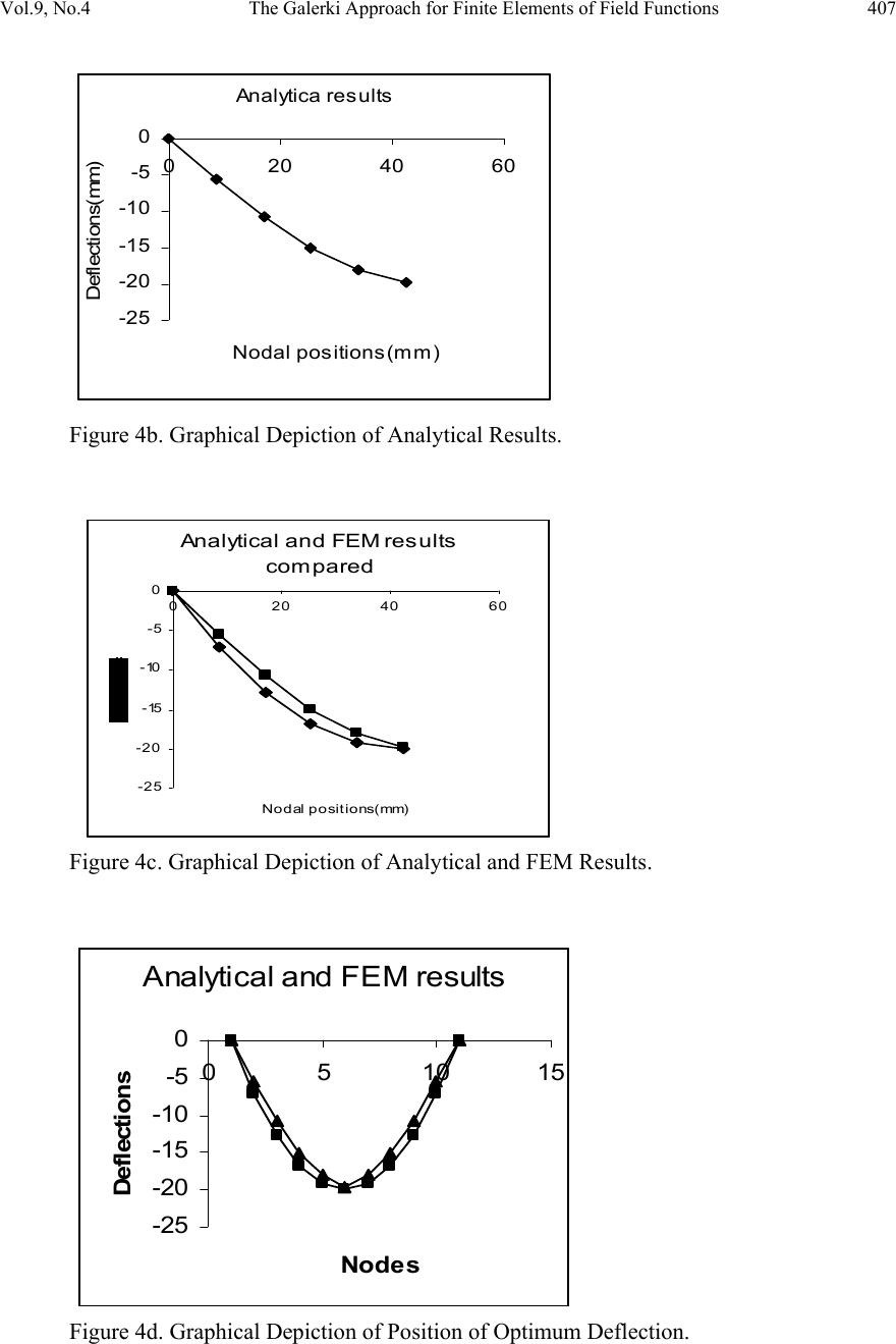

Vol.9, No.4 The Galerki Approach for Finite Elements of Field Functions 407
Analyt ic a r esult s
-25
-20
-15
-10
-5
0
0 204060
Nodal posit ions(mm)
Defle ctio ns( mm)
Figure 4b. Graphical Depiction of Analytical Results.
A
nalyt ic al and FEM result s
compared
-25
-20
-15
-10
-5
0
0204060
Noda l position s (mm)
Figure 4c. Graphical Depiction of Analytical and FEM Results.
Analyt ical and FEM r esul ts
-25
-20
-15
-10
-5
0
051015
Nodes
Deflections
Figure 4d. Graphical Depiction of Position of Optimum Deflection.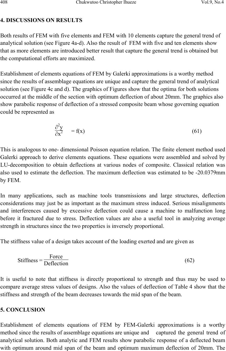

408 Chukwutoo Christopher Ihueze Vol.9, No.4
4. DISCUSSIONS ON RESULTS
Both results of FEM with five elements and FEM with 10 elements capture the general trend of
analytical solution (see Figure 4a-d). Also the result of FEM with five and ten elements show
that as more elements are introduced better result that capture the general trend is obtained but
the computational efforts are maximized.
Establishment of elements equations of FEM by Galerki approximations is a worthy method
since the results of assemblage equations are unique and capture the general trend of analytical
solution (see Figure 4c and d). The graphics of Figures show that the optima for both solutions
occurred at the middle of the section with optimum deflection of about 20mm. The graphics also
show parabolic response of deflection of a stressed composite beam whose governing equation
could be represented as
∂2y
∂x2 = f(x) (61)
This is analogous to one- dimensional Poisson equation relation. The finite element method used
Galerki approach to derive elements equations. These equations were assembled and solved by
LU-decomposition to obtain deflections at various nodes of composite. Classical relation was
also used to estimate the deflection. The maximum deflection was estimated to be -20.0379mm
by FEM.
In many applications, such as machine tools transmissions and large structures, deflection
considerations may just be as important as the maximum stress induced. Serious misalignments
and interferences caused by excessive deflection could cause a machine to malfunction long
before it fractured due to stress. Deflection values are also a useful tool in analyzing average
strength in structures since the two properties is inversely proportional.
The stiffness value of a design takes account of the loading exerted and are given as
Stiffness =
Force
Deflection (62)
It is useful to note that stiffness is directly proportional to strength and thus may be used to
compare average stress values of designs. Also the values of deflection of Table 4 show that the
stiffness and strength of the beam decreases towards the mid span of the beam.
5. CONCLUSION
Establishment of elements equations of FEM by FEM-Galerki approximations is a worthy
method since the results of assemblage equations are unique and captured the general trend of
analytical solution. Both analytic and FEM results show parabolic response of a deflected beam
with optimum around mid span of the beam and optimum maximum deflection of 20mm. The

Vol.9, No.4 The Galerki Approach for Finite Elements of Field Functions 409
maximum deflection, a measure of optimum instability for GRP composites is therefore
evaluated by this study as 20mm.
REFERENCES
[1] Hawkes, B. and Abinett, R., (1985). The Engineering Design Process, Pitman Publishing.
p101.
[2] Ihueze, C.C., (2005).Optimum Buckling Response Model of GRP Composites, Ph.D
Thesis, University of Nigeria. p111.
[3] Chapra, S.C and Canale, R.P., (1998). Numerical Methods for Engineers, McGraw-Hill
Publishers, 3rd edition, Boston, N.Y. p853.
[4] Astley, R.J., (1992). Finite Elements in Solids and Structures, Chapman and Hall
Publishers, UK. p154.
[5] Enetanya, A.N. and Ihueze, C. C., (2008). Computational Approaches for Strengths of
GRP Composites. Journal of Engineering and Applied Sciences, vol.4 No.1 and 2. P62.
[6] Black, P.H. and Adams, O.E., (1981).Machine Design. McGraw-Hill International Book
Company, Tokyo. p41.
[7] Benham, P.P. and Warnock, F.V., (1981). Mechanics of Solids and Structures.
Pitman Books, Toronto. p257.
[8] Beer, F. P. and Johnston, B., (1977). Vector Mechanics for Engineers (Statics), 3rd
edition. McGraw-Hill Book Company, New York. p354.
[9] Koshal, D., (1998). Manufacturing Engineers Reference Book, Butterworth Heinemann
Publisher. p102.
[10] Rosen, B.W., (1965). Mechanics of Composite Strengthening: Fibre Composite
Materials, American Society of Metals, Chapter 3.
[11] Kyriakides, S., Perry, E.J., and Liechti, K.M., (1994). Instability and failure of fibre
composites in compressive, ASME Journal of Applied Mechanics, Vol. 47, No. 6, S 262
– 266.
[12] Zienkiewicz, O.C., (1977). The Finite Element Method: Basic Formulation and Linear
Problems, 3rd ed., vol.1, McGraw-Hill, London. p228-301.