Journal of Minerals & Materials Characterization & Engineering, Vol. 9, No.4, pp.353-363, 2010
jmmce.org Printed in the USA. All rights reserved
353
Parametric Optimization of Gas Metal Arc Welding Processes by Using
Factorial Design Approach
Manoj Singla, Dharminder Singh, Dharmpal Deepak*
Department of Mechanical Engg., R.I.E.I.T.,Railmajra, 144533, INDIA
*Corresponding Author: [e-mail]
ABSTRACT
Gas Metal Arc Welding is a process in which the source of heat is an arc format between
consumable metal electrode and the work piece with an externally supplied gaseous shield of gas
either inert such as argon, helium. This experim ental s tudy aim s at optimizing various Gas Metal
Arc welding parameters including welding voltage, weld ing current, welding speed a nd nozzle to
plate distance (NPD) by developing a m athematical model for sound weld deposit area of a mild
steel specimen. Factorial design approach has been applied for finding the relationship between
the various process parameters and weld deposit area. The study revealed that the welding
voltage and NPD varies directly with weld deposit area and inverse relationship is found
between welding current and speed with weld deposit area.
Keywords: Gas Metal Arc Welding; Factorial Design Approach; Weld Deposit Area.
1. INTRODUCTION
Gas Metal Arc Welding is a process in which the source of heat is an arc format between
consumable metal electrode and the work piece, and the arc and the molten puddle are protected
from contamination by the atmosphere (i.e. oxygen and nitrogen) with an externally supplied
gaseous shield of gas either inert such as argon, helium or an argon-helium mixture or active
such as carbon dioxide, argon-carbon dioxide mixture, which is chemically active or not inert
(Karadeniz et al. 2007). Initially GMAW was called as MIG Welding because only inert gasses
were used to protect the molten puddle. The application of this process was restricted to
aluminum, deoxidized copper and silicon bronze. Later it was used to weld ferrite and austenitic
steels, and mild steel successfully by using active gasses in place of inert gasses and hence was
term MAG (Metal Active Gas) welding (Suban and Tusek, 2003, Quinn et al. 1999).
The American Welding Society refers to the process Gas Metal Arc Welding process to cover
inert as well as active shield gasses. GMAW is basically a semi automatic process, in which the

354 Manoj Singla, Dharminder Singh, Dharmpal Deepak Vol.9, No.4
arc lengths of electrode and the feeding of the wire are automatically controlled. The welding
operator’s job is reduced to positioning the gun at a correct angle and moving it along the seam
at a controlled travel speed. Hence less operator skill is required with this process as compare to
TIG and manual metal arc process. Yet basic training is required in the setting up of the
equipment and manipulation of the gun must be provided to the operator to ensure quality
GMAW welding (Jang et al. 2005, Praveen and Yarlagadda, 2005).
GMAW welding process overcome the restriction of using small lengths of electrodes and
overcome the inability of the submerged-arc process to weld in various positions. By suitable
adjusting the process parameters, it is possible to weld joints in the thickness range of 1-13 mm
in all welding position (Kuk et al. 2004, Murugan and Parmar, 1994)
All the major commercial metals can be welded by GMAW (MIG/CO2) process, including
carbon steels, low alloy and high alloy steels, stainless, aluminum, and copper titanium,
zirconium and nickel alloys. (Quintino and Allum, 1981, Smati, 1985)
GMAW (MIG/CO2) is also used in mechanized and automatic forms to eliminate the operator
factor and to increase the productivity and consistency of quality.
1.1 Mechanism of Metal Transfer in GMAW
In the GMAW (MAG) process, the metal transfer from the electrode tip to the weld pool across
the arc is either globular, spray type or short-circuiting type depending upon many factors, which
are enlisted as follows:
• The magnitude of welding current
• Shielding gas
• Current density
• Electrode extension and
• Electrode chemistry
With CO2 shielding, the globular and non-axial, whatever may be the value of the welding
current, current density and other factors. Hence there is considerable spatter. Drops become
smaller in size as the current increases and they continue to be directed axially and non-axially.
Axial transfer means that the metal droplets move along a line that is an extension of the
longitudinal axis of the electrode. Non-axial transfer means that the droplets are hurled in any
other directions. The non-axial transfer is caused by electromagnetic repulsive force acting on
the bottom of the molten drop. The electric current flowing through the electrode gives rise to
several electromagnetic forces that act on the motel tip including the pinch force (p) and the
anode reaction force (R). The pinch force which increases with current and electrode diameter
causes the drop to detach. With CO2 shielding, the electrode tip is not heated directly by the arc
plasma but by the arc heat conducted through the molten drop. The molten drop grow in size and

Vol.9, No.4 Parametric Optimization of Gas Metal Arc Welding Processes 355
finally detaches by short circuiting or gravity, after having overcome the force R, which tends to
support the drop.
1.2 Factorial Design Approach and Terminology
Factorial experiments permits to evaluate the combined effect of two or more experiments
variables when evaluated simultaneously. Information obtained from factorial experiments is
more complete than those obtained from a series of single factor experiments, in the sense that
factorial experiments permit the evaluation of interaction effects. An interaction effect is an
effect attributable to the combination of variables above and beyond that which can be predicted
from the variables considered separately.
For the need of factorial experiments, the information gathered could be used to make decisions,
which have a board range of applicability. In addition to information about how the experiments
variables operate in relative isolation, it can be predicted, what will happen when two or more
variables are used in combination. Apart from the information about interactions, the estimate of
the effects of the individual variables is a more practical use. In the case of factorial experiments,
the population to which inferences can be made is more inclusive than the corresponding
population for a single factor experiments. Factors may be classified as treatment and
classification factors.
• Classification factors group the experimental units into classes which are
homogeneous with respect to what is being classified.
• Treatment factors define experimental conditions applied to an experimental unit.
The administration of the treatment factors is under the direct control of the
experimenter, where as classification factors are not, in sense.
The effects of the treatment factors are of primary interest to the experimenter, where as
classification methods are included in an experiment to reduce experimental error and clarify
interpretation of the effects of the treatment factors.
The design of factorial experiments is concerned with answering the following questions:
• What factors should be included?
• How many levels of each factor should be included?
• How should the levels of the factors be spaced?
• How many experimental units should be selected for each treatment conditions?
• Can the effects of primary interests be estimated adequately from the experimental
data that will be obtained?
A factor is a series of related treatments or related classifications. The related treatments making
a factor constitute the levels of that factor. The number of levels within a factor is determined
largely by the thoroughness with which an experimental desires to investigate the factor.

356 Manoj Singla, Dharminder Singh, Dharmpal Deepak Vol.9, No.4
Alternatively, the levels of a factor determined by the kind of inference the experimental desires
to make upon a conclusion of experiment.
The dimensions of a factorial experiment are indicated by the number of levels of each factor.
For the case of p*q factorial experiment, PQ different treatment combinations are possible. As
number of factor increases, or as the number of levels with in a factor increases, the number of
treatment combinations in a factorial experiment increases quite rapidly.
In an experiment, the elements observed under each of the treatment combinations will generally
be a random sample from some specified population. This population may contain potentially
infinite number of elements. If n elements are to be observed under each of treatment
combination in p*q factorial experiment, a random sample of npq elements from population is
required. The npq elements are then subdivide at random to the treatment combinations.
The P potential levels may be grouped in to P levels (p<q) by either combining adjoining levels
or deliberately selecting what are considered to be representative levels.
When p = P then the factor is called the fixed factor. When the selection of the p levels from the
potential P levels is determined by some systematic, non-random procedure, then also the factor
is considered a fixed factor. In this later case, the selection procedure, reduce the potential P
levels to p effective levels .Under this type of selection procedure, the effective, potential
number of levels of factor in the population may be designated as P effective and P effectiv e = p.
In contrast to this systematic selection procedure, if the p levels of factor A included in the
experiment represents a random sample from the potential p levels, then the factor is considered
to be random factor. In most practical situations in which random factors are encountered, p is
quite small to relative to P, and the ratio p/P is quite close to zero.
The ratio of the number of levels of a factor in an experiment to the potential number of levels in
the population is called the sampling fraction for a factor. In term of this sampling fraction, the
definition of fixed and random factors may be summarized as mentioned in Table 1.
Table 1. Relationship between Sampling Fraction and Fixed Random Factors
Sampling fraction Factor
p/P or p/Peffective =1 A is a fixed factor
p/P = 0 A is a random factor
Cases in which the sampling fraction assumes a value between 0 and 1 do occur in practice.
However, cases in which sampling fraction is either 1 or very close to 0 encountered more
frequently. Main effects are defined in terms of parameters. Direct estimates of these parameters
will be obtainable for corresponding statistics.

Vol.9, No.4 Parametric Optimization of Gas Metal Arc Welding Processes 357
The main effect for the level is the difference between the mean of all potential observations on
the dependent variable at the level and grand mean of all potential observations.
The interaction between different levels is a measure of the extent to which the criterion mean
for treatment combination cannot be predicted from the sum of the corresponding main effects.
From many points of views, the interaction is a measure of the non-addivity of the main effects.
To some extent the existence or non-existence of interaction depends upon the scale of
measurement. For example, the interaction may not be present in terms of a logarithmic scale of
measurement, whereas in terms of some other scale of measurement an interaction may be
present. If alternative choices are present, then that scales which leads to the simplest additive
model will generally provide the most complete and adequate summary of the experimental data.
2. METHODOLOGY
For this project, after conducting the related literature survey we found that the among the most
important parameters were voltage, current , speed of arc travel and , nozzle to plate distance
while keeping the wire diameter constant, which is 1.2 mm in this case. So these four variables
were used as treatment variables for the model.
2.1 Treatment Variables:
• Voltage (V)
• Current (I)
• Speed(S)
• Nozzle To Plate Distance (NPD)
For conducting trial runs values or levels of these variables were chosen randomly from an
infinite potential level i.e. the sampling fraction for these trials runs was equal to zero, however,
we got a rough range of these factors from the literature we surveyed. With the help of these
trials runs effective, representative’s levels were developed for each factor (variables).
The numbers of levels for to be included in the experiment were chosen for each factor as per the
design. These numbers of levels were two for each so as per the definition it is a 2n (2*2*2*2)
factorial experiment. Where n is number of factors. If full factorial approach had been practiced,
the number treatment combination would have been 16. But without affecting the accuracy of the
model and the objective of the test we went for half factorial approach according to which the
number of treatment combinations becomes 2n-1 (24-1 = 23 = 8). The levels for each factor were
the highest value and the lowest value of the factors in between and at which the outcome was
acceptable. These values were outcomes of trials runs. Highest value has been represented by ‘+’
and the lowest value has been represented by ‘-’ as mentioned in Table 2. As per the design
matrix the final runs were conducted and the response i.e. the weld deposit area was measured
and noted down against each combination.
Then the values of different coefficients were calculated as per the modeling. These values of
coefficients represent the significance of corresponding factors (variable) on the response.

358 Manoj Singla, Dharminder Singh, Dharmpal Deepak Vol.9, No.4
Higher the value of coefficients, higher the influence of the variable on the response. Negative
value of coefficients indicates the inverse relationship between variable and response.
The calculation was done as per the following model.
2.2 Design Matrix
Table 2. Model Showing the treatment variables
S. No. Voltage (V)
X1 Current (I) X2Speed (S) X3 Nozzle to plate
difference (NPD) X4
1. + + + +
2. - + + -
3. + - + -
4. - - + +
5. + + - -
6. - + - +
7. + - - +
8. - - - -
2.3 Mathematical Model Developed
Assuming the values of responses as y1, y2, y3, y4, y5, y6, y7, y8 against the treatment
combinations 1, 2, 3, 4, 5, 6, 7, 8 respectively (as per the S. No. in the matrix design) Y as the
optimized value of response (i.e. left hand side in the equation used for the showing the relation
among the factors and the response).
Relation between main effects interactions effects and the response has been shown in the
following equation:
Y = b0 + b1X1 + b2X2 + b3X3 + b4X4 + b12(X1X2) + b13(X1X3) + b14(X1X4) + b23(X2X3) +
b24(X2X4) + b34(X3X4)
Here Y is the optimized weld deposit area, yi (i = 1 to 8) is the response of the ith treatment
combination, b0 is the mean of all the responses, bj (j =1 to 4) is the coefficient of jth main factor (j
= 1 for voltage, 2 for current, 3 for speed, 4 for NPD), and bjk( j, k=1 to 4) is the coefficient for
interaction factor.

Vol.9, No.4 Parametric Optimization of Gas Metal Arc Welding Processes 359
Values of all these coefficients were calculated as followings:
b0 =
∑ yi / 8
= [(y1+y2+y3+y4+y5+y6+y7+y8)]/8
b1 = [(y1-y2+y3-y4+y5-y6+y7-y8)]/8
= [(y1+y3+y5+y7)-(y2+y4+y6+y8)]/8
b2 = [(y1+y2-y3-y4+y5+y6-y7-y8)]/8
[(y1+y2+y5+y6) - (y3+y4+y7+y8)]/8
b3 = [(y1+y2+y3+y4-y5-y6-y7-y8)]/8
= [(y1+y2+y3+y4) - (y5+y6+y7+y8)]/8
b4 = [(y1-y2-y3+y4-y5-y6+y7-y8)]/8
= [(y1+y4+y6+y7) - (y2+y3+y5+y8]/8
b12 = [(y1-y2+y3+y4+y5+y6+y7+y8)]/8
= [(y1+y4+y5+y8) - (y2+y3+y6+y7)]/8
b13 = [(y1-y2+y3-y4-y5+y6-y7+y8)]/8
= [(y1+y3+y6+y8) - (y2+y4+y5+y7)]/8
b14 = [(y1+y2-y3-y5-y6+y7+y8)]/8
= [(y1+y2+y7+y8) - (y3+y4+y5+y6)]/8
b23 = [(y1+y2-y3-y4-y5 - y6+y7+y8)]/8
= [(y1+y2+y7+y8) - (y3+y4+y5+y6)]/8
b24 = [(y1-y2+y3-y4-y5+y6-y7+y8)]/8
= [(y1+y3+y6+y8)-(y2+y4+y5+y7)]/8
b34 = [(y1-y2-y3+y4+y5-y6-y7+y8)]/8
= [(y1+y4+y5+y8) - (y2+y3+y6+y7)]/8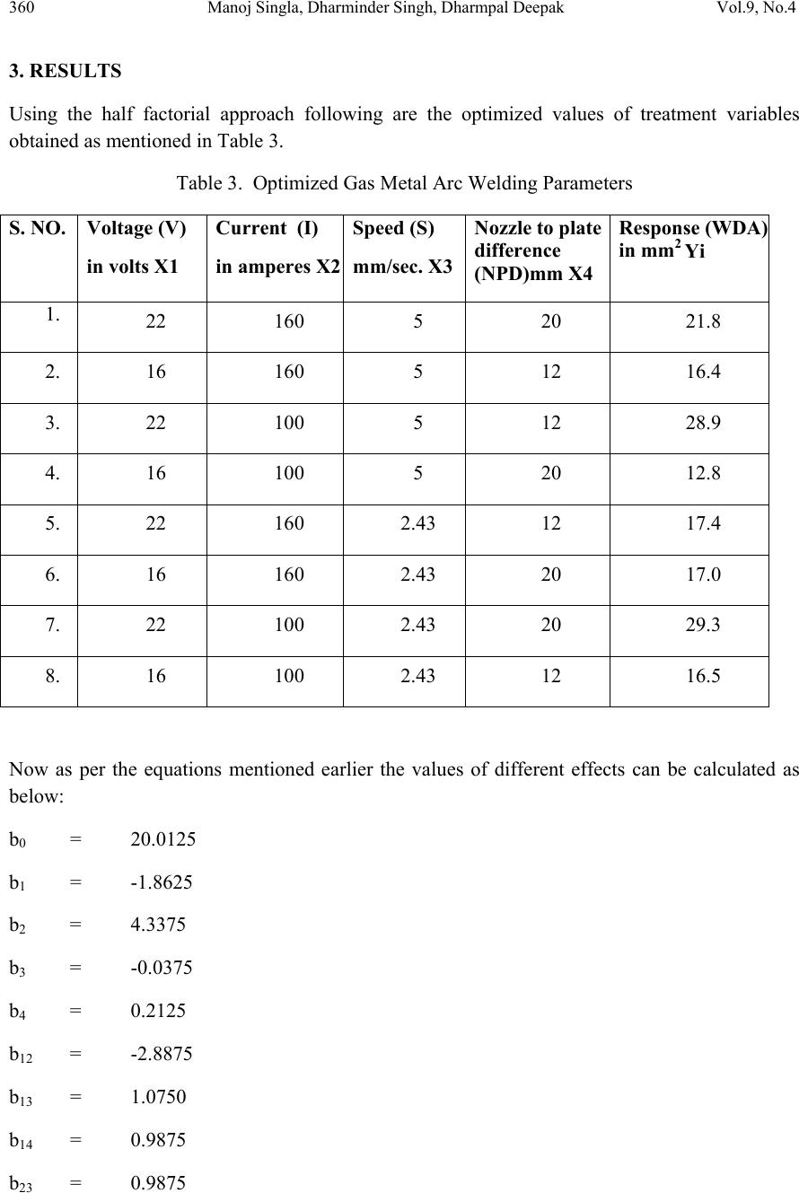

360 Manoj Singla, Dharminder Singh, Dharmpal Deepak Vol.9, No.4
3. RESULTS
Using the half factorial approach following are the optimized values of treatment variables
obtained as mentioned in Table 3.
Table 3. Optimized Gas Metal Arc Welding Parameters
S. NO. Voltage (V)
in volts X1
Current (I)
in amperes X2
Speed (S)
mm/sec. X3
Nozzle to plate
difference
(NPD ) mm X4
Response (WDA)
in mm2 Yi
1. 22 160 5 20 21.8
2. 16 160 5 12 16.4
3. 22 100 5 12 28.9
4. 16 100 5 20 12.8
5. 22 160 2.43 12 17.4
6. 16 160 2.43 20 17.0
7. 22 100 2.43 20 29.3
8. 16 100 2.43 12 16.5
Now as per the equations mentioned earlier the values of different effects can be calculated as
below:
b0 = 20.0125
b1 = -1.8625
b2 = 4.3375
b3 = -0.0375
b4 = 0.2125
b12 = -2.8875
b13 = 1.0750
b14 = 0.9875
b23 = 0.9875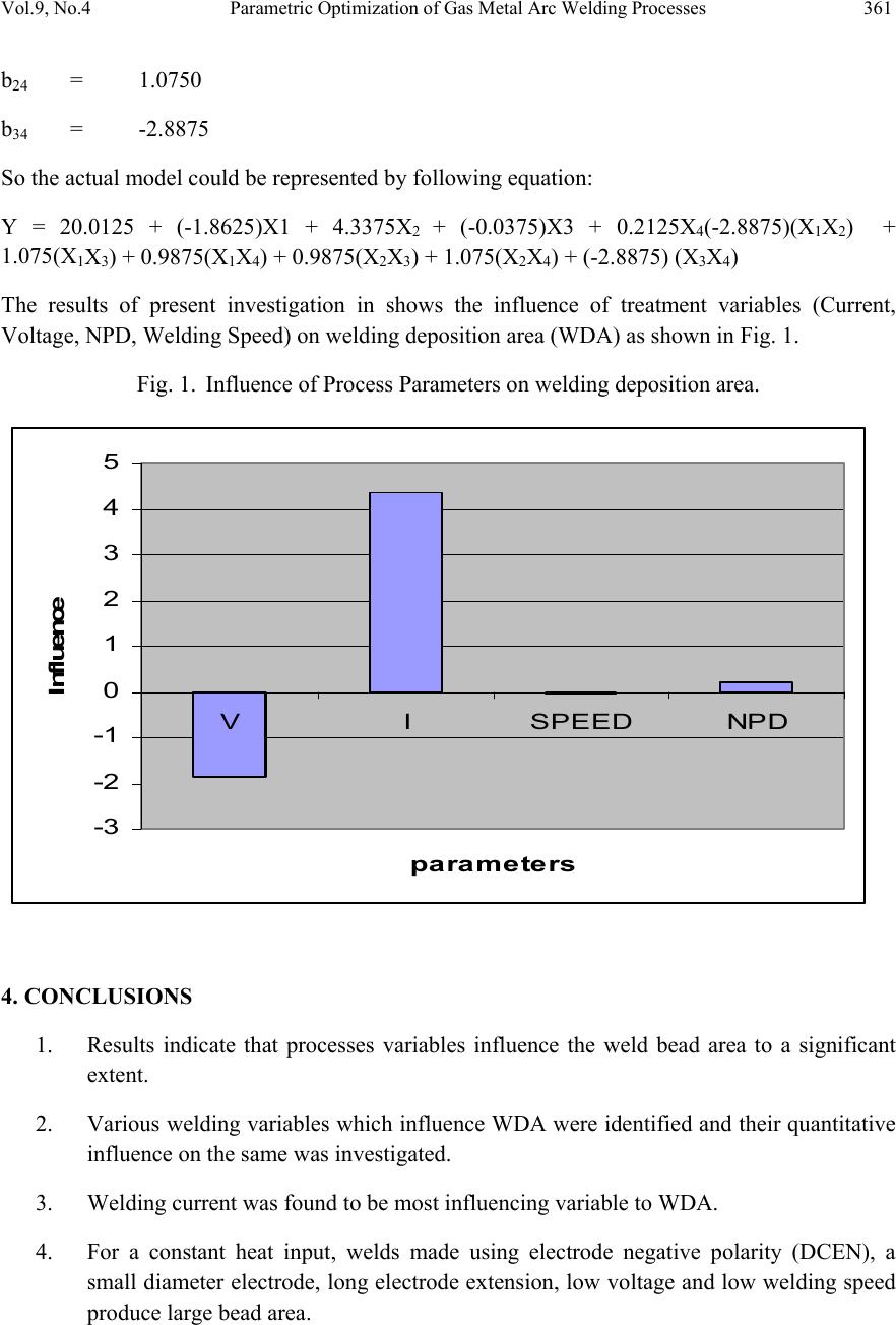

Vol.9, No.4 Parametric Optimization of Gas Metal Arc Welding Processes 361
b24 = 1.0750
b34 = -2.8875
So the actual model could be represented by following equation:
Y = 20.0125 + (-1.8625)X1 + 4.3375X2 + (-0.0375)X3 + 0.2125X4(-2.8875)(X1X2) +
1.075(X1X3) + 0.9875(X1X4) + 0.9875(X2X3) + 1.075(X2X4) + (-2.8875) (X3X4)
The results of present investigation in shows the influence of treatment variables (Current,
Voltage, NPD, Welding Speed) on welding deposition area (WDA) as shown in Fig. 1.
Fig. 1. Influence of Process Parameters on welding deposition area.
-3
-2
-1
0
1
2
3
4
5
VISPEED NPD
parameters
Influence
4. CONCLUSIONS
1. Results indicate that processes variables influence the weld bead area to a significant
extent.
2. Various welding variables which influence WDA were identified and their quantitative
influence on the same was investigated.
3. Welding current was found to be most influencing variable to WDA.
4. For a constant heat input, welds made using electrode negative polarity (DCEN), a
small diameter electrode, long electrode extension, low voltage and low welding speed
produce large bead area.

362 Manoj Singla, Dharminder Singh, Dharmpal Deepak Vol.9, No.4
5. The two level fractional half area fractional designs is found to be very effective tool
for quantifying to main and interaction effects of variable on weld bead area.
6. The model is problem specific however the technique can be applied very effectively.
ACKNOWLEDGEMENT
The author acknowledges with thanks the support provided by Department of Mechanical
Engineering, RIEIT, Railmajra, Distt. Nawanshahr (PB) India.
REFERENCES
1. E. Karadeniz, Ozsarac, U. and Yildiz, C., “The effect of process parameters on
penetration in gas metal arc welding process”, Materials and Design, 2007 , Vol 28 ,
Issue 2 , pp. 649-656.
2. M. Suban and J. Tusek, “Methods for the determination of arc stability”, Journal of
Materials Processing Technology, 2003, pp. 430-437.
3. T.P. Quinn, C. Smith, C.N. McCowan, E. Blachowiak, R.B. Madigan, “Arc Sensing for
Defects in Constant-Voltage Gas Metal Arc Weldiing”, Welding Journal, 1999, Vol. 78,
pp. 322-328.
4. P. J. Hewitt and M. G. Madden, “Chromium in welding process parameters and
hexavalent MIG Fume.”, Ann. Occup. Hyg.,1986, Vol. 30, No. 4, pp. 427-434.
5. K.C. Jang, D.G. Lee, J.M. Kuk and I.S. Kim, “Welding and environmental test condition
effect in weldability and strength of Al alloy”, Journal of Materials Processing
Technology, 2005, Vol. 164-165, pp.1038-1045.
6. P. Praveen, P.K.D.V. Yarlagadda, “Meeting challenges in welding of aluminum alloys
through pulse gas metal arc welding”, Journal of Materials Processing Technology, 2005,
pp.1106-1112.
7. J. M. Kuk, K. C. Jang, D. G. Lee, I. S. Kim, “Effects of temperature and shielding gas
mixture on fatigue life of 5083 aluminum alloy”, Journal of Materials Processing
Technology, 2004, Vol. 155-156, , pp.1408-1414.
8. N. Murugan, R. S. Parmar, “Effects of MIG process parameters on the geometry of the
bead in the automatic surfacing of stainless steel”, Journal of Materials Processing
Technology, 1994, Vol. 41, pp. 381-398.
9. P. Praveen, P.K.D.V. Yarlagadda, M.J. Kang, “Advancements in pulse gas metal arc
welding”, Journal of Materials Processing Technology, Vol. 164-165, 2005, pp.1113-
1119.

Vol.9, No.4 Parametric Optimization of Gas Metal Arc Welding Processes 363
10. L. Quintino and C.J. Allum, “Pulsed GMAW: interactions between process parameters –
part 1”, Welding Met. Fabrication, Vol. 85, 1981, pp. 5–9.
11. S. Ueguri, K. Hara, H. Komura, “Study of metal transfer in pulsed GMA welding”, Weld.
J., 1985, Vol. 64, pp. 242–50.
12. Z. Smati, Automated pulsed MIG welding, Metal Construction, 1985, Vol. 18, pp 38–44.
13. Y. S. Kim, “Metal transfer in gas metal arc welding”, PhD Thesis, 1989, MIT: USA.
14. J. H. Waszink, M. J. Piena, “Experimental investigation of drop detachment and drop
velocity in GMAW”, Welding Journal , Vol. 65 ,1986 , pp.289–98.
15. L. A. Jones, T. W. Eager, J. H. Lang, “Magnetic forces acting on molten drops in gas
metal arc welding”, J. Phys. D. Appl. Phys., Vol. 31 ,1998, pp. 93-106.
16. J. H. Nixon, J. Norrish, “Determination of pulsed MIG process parameters”, Welding and
Metal Fabrication, 1988 , pp. 4-7.
17. F. Wang, W. K. Hou, S. J. Hu, E Kannatey-Asibu, W. W. Schultz, P. C. Wang,
“Modelling and analysis of metal transfer in gas metal arc welding”, J. Phys. D: Appl.
Phys., Vol. 36 , 2003 , pp.1143-1152.
18. F. Zhu, “A comprehensive dynamic model of the gas metal arc welding process”, PhD
Thesis, 2003, University of Missouri- Rolla USA .
19. M. Goodarzi, “Mathematical modelling of gas tungsten arc welding (GTAW) and gas
metal arc welding (GMAW) processes”, PhD Thesis, 2003, University of Toronto
Canada.
20. Ghosh P.K., Gupta S.R., Gupta P.C., Rathi R., “Fatigue characteristics of pulsed MIG-
welded Al-Zn-Mg alloy”, Journal of Material Science , Vol. 26 , Issue 22 ,1991, pp.
6161-6170.