Open Journal of Statistics, 2012, 2, 356-367
http://dx.doi.org/10.4236/ojs.2012.23044 Published Online July 2012 (http://www.SciRP.org/journal/ojs)
Prediction Based on Generalized Order Statistics from a
Mixture of Rayleigh Distributions Using
MCMC Algorithm
Tahani A. Abushal1, Areej M. Al-Zaydi2
1Department of Mathematics, Umm Al-Qura University, Makkah Al-Mukarramah, KSA
2Department of Mathematics, Taif University, Taif, KSA
Received May 15, 2012; revised June 16, 2012; accepted June 30, 2012
ABSTRACT
This article considers the problem in obtaining the maximum likelihood prediction (point and interval) and Bayesian
prediction (point and interval) for a future observation from mixture of two Rayleigh (MTR) distributions based on
generalized order statistics (GOS). We consider one-sample and two-sample prediction schemes using the Markov
chain Monte Carlo (MCMC) algorithm. The conjugate prior is used to carry out the Bayesian analysis. The results are
specialized to upper record values. Numerical example is presented in the methods proposed in this paper.
Keywords: Mixture Distributions; Rayleigh Distribution; Generalized Order Statistics; Record Values; MCMC
1. Introduction
The concept of generalized order statistics GOS was in-
troduced by [1] as random variables having certain joint
density function, which includes as a special case the
joint density functions of many models of ordered ran-
dom variables, such as ordinary order statistics, ordinary
record values, progressive Type-II censored order statis-
tics and sequential order statistics, among others. The
GOS have been considered extensively by many authors,
some of them are [2-18].
In life testing, reliability and quality control problems,
mixed failure populations are sometimes encountered.
Mixture distributions comprise a finite or infinite number
of components, possibly of different distributional types,
that can describe different features of data. In recent years,
the finite mixture of life distributions have to be of con-
siderable interest in terms of their practical applications in
a variety of disciplines such as physics, biology, geology,
medicine, engineering and economics, among others.
Some of the most important references that discussed dif-
ferent types of mixtures of distributions are [19-25].
Let the random variable follows Rayleigh lifetime
model, its probability density function (PDF), cumulative
distribution function (CDF) and reliability function (RF)
are given below:
T
 
0,0,t  
 
0,0,t   

2,
t
Rt e
 


2,ht te 

2
1,
t
Ht e
 

2
t   (1)
(2)
(3)
Also, the hazard rate function (HRF)


2,tt (4)

 






where ....hR
 
The cumulative distribution function (CDF), denoted
by


H
t, of a finite mixture of k components, denoted
by


,1,,
j
H
tj k
 
1
,
k
jj
j
is given by
H
tpHt


1, ,jk
(5)
where, for

0p
1.
kp the mixing proportions j
and 1j
j

2k
p1pp
The case of , in (5), is practical
importance and so, we shall restrict our study to this case.
In such case, the population consist of two sub-popula-
tions, mixed with proportions 1 and 21

. In
this paper, the components are assumed to be Rayleigh
distribution whose PDF, CDF, RF and HRF are given,
respectively, by




112 2
htph tpht (6)


112 2,
H
tpHtpHt (7)


112 2,RtpR tpRt (8)




,thtRt  
1, 2j
(9)
where, for

, the mixing proportions
j
p are such
C
opyright © 2012 SciRes. OJS

T. A. ABUSHAL, A. M. AL-ZAYDI357
01that 12jand, 1ppp






,,
j
HtRt
jj are
given from (1)-(3) after using
ht
j

instead of

.
Several authors have predicted future order statistics
and records from homogeneous and heterogeneous popu-
lations that can be represented by single component dis-
tribution and finite mixtures of distributions, respectively.
For more details, see [9,10,26].
Recently, a few of authors utilized the GOS’s in Bayes-
ian inference. Such authors are [7-9,18]. Bayesian infer-
ences based on finite mixture distribution have been dis-
cussed by several authors such that: [23,24,27-33].
For Bayesian approach, the performance depends on
the form of the prior distribution and the loss function
assumed. A wide variety of loss functions have been de-
veloped in the literature to describe various types of loss
structures. The balanced loss function was suggested by
[34]. [35] introduced an extended class of the balanced
loss function of the form
 
  
0
,
,1


0
,,
L

 
,,

      
 


.
 
,
 (10)
where is a suitable positive weight function and


 

is an arbitrary loss function when estimate-
ing

 by

. The parameter 0

is a chosen prior
estimator of



0
, obtained for instance from the crite-
rion of maximum likelihood (ML), least squares or unbi-
asedness among others. They give a general Bayesian
connection between the case of and
0


,0,
kk
r
where . 01


,,mm

n
Suppose that
1;,, 2;,,;,,
,,,
nmk nmkrnm
TT T


1,,, r
r
Rm m



1r
tt  

R
11 11 r 
are the first
(out of ) GOS drawn from the mixture of two Ray-
leigh MTR distribution. The likelihood function (LF) is
given in [1], for by
m

 
1
1
i
m
r
ri
iRt ht









,
r
t  
1
1
,
.
r
rii
i
n
i
Ck
Mi











i
Rt
 
1,
r
irr
t ht
 


1
0,
i
i
niM

i
p
1
,,
LtC R  
(11)
where , is the parameter space,
and
tt
1 (12)
where and are given, respectively, by (5)
and (7).

ht
The purpose of this paper is to obtained the maximum
likelihood prediction (point and interval) and the Bayes
prediction (point and interval) in the case of one-sample
scheme and two-sample scheme. The point predictors are
obtained based on balanced square error loss (BSEL)
function and the balanced LINEX (BLINEX) loss func-
tion. We used ML to estimate the parameters, and
j

of the MTR distribution based on GOS. The conju-
gate prior is assumed to carry out the Bayesian analysis.
The results are specialized to the upper record values. The
rest of the article is organized as follows. Section 2 deals
with the derivation of the maximum likelihood estimators
of the involved parameters. Sections 3 and 4, deals with
studying the maximum likelihood (point and interval) and
the Bayes prediction (point and interval) in the case of
one-sample scheme and two-sample scheme. In Section 5,
the numerical computations results are presented and the
concluding remarks.
2. Maximum Likelihood Estimation (MLE)
Substituting (6), (7) in (11), the LF takes the form

 
 
 
1
112 2
1
112 2
1
1
1122.
i
r
m
r
ii
i
r
ii
i
rr
LtpRt pRt
ph tpht
pR tpRt






 

 







(13)
Take the logarithm of (13), we have


 
 
 
1
1122
1
112 2
1
1122
ln ln
+ln
1ln ,
r
iii
i
r
ii
i
rrr
lLtmpRtpRt
ph tpht
pR tpRt





  




 



,1pppp
(14)
where 12

 p . Differentiating (14) with re-
spect to the parameters and
j

and equating to zero
gives the following likelihood equations
  
 
 
1**
11
1
1**
1
10,
10,
1, 2
rr
iiirr
ii
r
jjiji
i
j
r
iji rjr
i
lmt tt
p
lptt
mt t
j































1, 2j
(15)

where, for
  
   
 
   

121 2 *
2
*
2
,,
,,
1
iii i
ii
ii
ji iji
ji ji
ii
ji i
j
ht htRtRt
tt
ht Rt
ht tRt
tt
ht Rt
tt












(16)












T. A. ABUSHAL, A. M. AL-ZAYDI 358
p
Equations (15) do not yield explicit solutions for
and
j

, and have to be solved numerically to
obtain the ML estimates of the three parameters. New-
ton-Raphson iteration is employed to solve (15).
1, 2j
,,TT 
n
Remark: The parameters of the components are as-
sumed to be distinct, so that the mixture is identifiable.
For the concept of identifiability of finite mixtures and
examples, see [19,36,37].
3. Prediction in Case of One-Sample Scheme
Based on the informative 1; ,,;,,nmk rnmk

GOS’s from
the MTR distribution, for the remaining unobserved
future () components, let ;, ,
r
s
nmk
T, s = r + 1, r +
2, denote the future lifetime of the ,nth
s
component
to fail,


1
s
nr, the maximum Likelihood pre-
diction (point (MLPP) and interval (MLPI)), Bayesian
prediction (point (BPP) and interval (BPI)) can be ob-
tained.
The conditional PDF of ;, ,
s
snmk
TT
 given that the
components that had already failed is

;, ,rrnmk
TT


 
  
 
  
1
*
1
1
1
1
1
1
ln ln
1!
,1,
(1) 1!
sr
sr
srr s
kk
srs

1
1
1
,1,
sr
s
r
m
rs
srs
Rt
RtRtht m

m
s
sr r
k
kttRt Rt
sr
RtRtht m
CRt
msrC












 
 
1m







  
 



 
(17)
In the case when , substituting (6) and (7) in
(17), the conditional PDF takes the form

  
 
 
 
*
1
1
112 211
112 2
1
112 2
ln
ln ]
sj
k
ss
rr
sr
ss
kt
pRt pRtpRt
pR tpRt
pR tpRt

2 2
112 2,.
k
rr
sssr
pRt
phh ttt


t p


  



 










1m
(18)
And in the case when , substituting (6) and (7)
in (17), the conditional PDF takes the form






*
21 1
112 2
11 2
112 2
sj s





1
1
22
1
2
1
1
112 2.,
s
r
s
rr
m
rr
s
r
m
ss
s
ssr
t
t
t
t
ttt























(19)
In the following, we considered two cases: the first is
when the mixing proportion p is known and the second
is when the two parameters
ktpRtpR
pR tpR
pR tpR
pR tpR
ph tph
 







and p are assumed to
be unknown.
3.1. Prediction When p Is Known
In this section we estimate 1 and 2


, assuming that
the mixing proportion, 1 p and 2 p are known.
3.
n
p r
1.1. Maximum Likelihood Prediction
Maximum likelihood predictio can be obtain using (18)
and (19) by replacing the shape arametes 1

and 2

by

1
ˆ
M
L
 and

2
ˆ
M
L
 which is obtained from (15).
1) Interval prediction
The MLPI for any future observation
s
t, s = r + 1, r +
2,, n can be obtained by
 


 

*
212
ˆˆ
,d
ss
ML ML
kt t 

*
112
ˆˆ
Pr,d ,1,
sss
ML L
v
tk tm 

,1.
M
t
m
v

 



t

(20)

A


1 100%   MLPI (L,U) of the futu observ-
tion
re a
s
t iby snear s given olving the following two nonli
equations

P) 2
s
tr1, Pr(.
2
s
tLtt tUt




 (21) 
2) Point prediction
The MLPP for any future observation ,
s
t s =
+2,,n can be obtained by replacing the shape pa-
rameters 1
r + 1, r
by ˆ

1
M
L

2
and

2

 and ˆ
M
L

 which, ob-
tained from (15)

 




112
*
212
,d ,1,
ˆˆ
,d,1
ss s
ML ML
v
ss ML ML
v
Etkt tm
kt tm



*ˆˆ
ˆsML
t
.





 (22)
3.1.2. Bayesian Prediction
When the mixing proportion, p is known. Let the para-
meters
j

,1, 2j

have a gamma prior distribution
with PDF
 
1
1
π,,, 0.
Γ()
jj jj
jjjjjj
j
e
 



 (23)
These are chosen since they are the conjugate priors
for the individual parameters. The joint prior density
function of


12
,

  is given by





1
π,

2
1
112 2
21
πππ,
j
j
jj
j
je








(24)



where


1, 2, 0, ,0.
jjj
j  


T. A. ABUSHAL, A. M. AL-ZAYDI359
It then follows, from (13) and (24), that th
ven by

e joint
posterior density function is gi

 
2
1 1
*
11
1
1122
2
πjj
j
jj
i
j
j
m
i
tA e
R tpR











 
 
1
1
11 2 2
1
1
112 2
]
r
r
i
i
r
ii
i
rr
pt
ph tpht
pR tpRt













 (25)
where



1πd.ALt

1


 (26)
The Bayes predictive density functi

on can be obtained
using (18), (19) and (25) as follow:
 

 

*
1
*
112
0
d, 1,
d,
ssj
ssj
Qtttkt m
Qtttkt m








1) Interval prediction
iction interval, for the future observation
**
11
0
**
π
π1.
(27)
Bayesian pred
;,,,
s
nmk
T 1,2, ,
s
rr n can be computed by ap- 
proximated

1s
Qtt using the MCM
[17,24], using the form
*C algorithm, see




1
*
1
*i
s
i
s
1
,
*d
s
r
j
i
j
s
itktt



 (28)
kt
Qtt





where

is the number of generated parameters and
i
j

, i1, 2,3,,

. They are generated from the poste-
rio) using Gibbs sampler and Me-
1 100%  BPI (L,
r density function (25
tro
A
polis-Hastings techniques, for more details see [38].

 U) of the future observation
s
t is given byg the following two nonlinear equa-
tions
solvin



*
1
*
1r it
d
1,
2
d
i
sjs
iL
i
sjs
kt t
kt t










 (29)



*
1
*
1
d
.
2
d
r
i
sjs
iU
i
sjs
it
kt t
kt t











 (30)
Numerical methods are generally necessary to solve
the above two equ
gi
ations to obtain L and U for a
ven

.
2) Point prediction
a) BPP for the future observation
s
t based on BSEL

function can be obtained using
 

1,
s
Ett (31)
where

sB S sML
tt 

s
ML
t
 is the ML prediction for future obser-
vation
the
s
t which can be obtained using (22) and

s
Ett
can be obtained using
 
*
Qd.
1
r
s
sss
t
b) BPP for the future observation
Etttttt

 (32)
s
tBLINX
loss functio
based on
n can be obtained using




1ln 1,
sML s
at at
sBL
te et
a

E


 





 (33)
where

s
ML
t
 is the ML prediction for the
vation
future obser-
s
t which can be obtained using (22) and


t c
s
at
Ee
an be obtained using



*
1d.
s
r
at
s
at
s
s
teQ ttt

 (34)
3.2. Prediction When p and θj Are Unknown
We
Ee t


hen both of the two parameters thmixing proportion
j
p and ,1,2
jj


, are assumed to be unknown.
3.2.1. Maximum Likelihood Prediction
Maximum likelihood prediction can be obtain using (18)
) byand (19 replacing the parameters p, 1

and 2

by
 
1
ˆ
,
ˆ
M
LML
p  and

2
ˆ
M
L
 which we obtained using
(15).
1) Interval prediction
The MLPI for any future observation ,
s
t1,
s
rr


2,, n can be obtained by

 


 

*
212
ˆˆ
ˆ,, d,1.
v
ss
ML ML ML
vktp tm


*
112
ˆˆ
ˆ
Pr,,d ,
ss s ML MLML
tt ktptm 
1,


 



(35)

A


1 100%   MLPI (L,U) of the future observa-
tion
s
t is given by solving the following two nonliner
Equations (1).
2) Piction
a
2
oint pred
e observation , The MLPP for any futur
s
t 1,
s
rr

2,,n

 can be obtained by replacing
p, 1
the shape pa-
rameters

and 2

by ˆ
, ˆ
 
1
M
LML
and

2
ˆ
p 
M
L

which, obtained from


(15).

 

 

*
112
*
212
ˆˆ
ˆˆ,,d, 1,
ˆˆ
ˆ,, d,1.
sss s sMLML MLML
t
ss s
ML MLML
t
tEttktp tm
tkt ptm









(36)

3.2.2. Bayesian Prediction
Let
j
p and ,1,2j
j


, are independent random vari-
ab


,Betabb and for1, 2, les such that 12 ~pj
j


to
foon ith PDF llow an inverted gamma prior distributiw

T. A. ABUSHAL, A. M. AL-ZAYDI 360
  
,, ,
jj
 
 (37)
A joint prio
1
10.
Γ
j jj
jj
j
jjj
j
j
pe
 


 








r density function of


12
,,p

  is
then given by
 



2
1
32
1
π,
,
j
12
121
11
1
2
2
πππ
π1
j
j
jj
e






1,p
bb j
p
pp




j
1
(38)
wher 12 1 0p p and for 1,20,
j
j e



,, 0.
jjj
b  
Using the likelihood function (13) and the prior density
function (38), the posterior density function will be in the
form

 
   
*
2
1
1
112 2
1
112 21122
1
π,
i
j
j
m
r
ii
i
r
iir r
i
pt
e
pR tpRt
ph tphtpR tpRt





 




 



9)

1,
r
 

2
1
12 1
11
21 2
2
jj
j
jj bb
Ap p






 

(3
where



1
2πd.ALt



 (40)
The Bayes prediction density function of
TT

,, ,snmk can be obtained,
ssee [39], by





1
0
*
2
**
21
0
**
1
22
π,,
π,,
s
sj
sj
Qtt
ptkt p
ptkt p






0
0
dd,1,
dd,1.
p m
p m




(41
1) Interval prediction
ction interval, for the future observ
)
ation Bayesian predi
;,,,
s
nmk
T 1,2, ,
s
rr n can be computed by ap- 
proximated

s
Qtt using the MCMC algorithm, see
[24], using the form
*
2




*
1
*
,
,
,d
ii
sj
i
ii
*
2
1r
s
s
js
it
Qt t

 (42)
1,2,3,,
kt p
kt p t








where ,,
ii
jpi

 are generated from the
ing Gibbs sampler an

1 100%   BPI (L,U)
pos-
d Me- terior density f
tropolis-Hastin
of the futu
unction (39) us
gs techniques. A
re observation
s
t is given by solving the fol-
s lowationing two nonlinear equ



*
*
,d
1,
2
,d
ii
sj s
ii
sj s
ktp t
tp t


1
1
r
iL
i
tk





, (43)





*
k


1
1*
,d
,
2
,d
r
ii
sj s
iU
iii
sj s
t
tp t
ktp t







 (44)
Numerical methods are generally necessary to solve
ve two equations


the aboto obtain L and U for a
given

.
1) Point prediction
BPP for the future observation
s
t based on BSEL
function can be obtained using


 

1,
s
sBSsML
tt Ett 
 (45)
where

s
ML
t
 is the ML prediction for the
vation
future obser-

s
t which can be obtained using (36) and

s
Ett
can be obtained using
 
*
2
Qd
r.
s
ss
t
Etttttt


2) BPP for the future observation
s
(46)
s
t based on BLINX
loss function can be obtained using




1,
sML s
lnne Eet
1at at
s
t
BLa






 (47)
w


here

s
ML
t
 is the ML prediction fr the future obser-
vation
o
s
t which can be obtained using (36) and


s
Ee t can be obtained using
at



*
ss
at at
2.d
r
s
s
t
EeteQttt (48)
4. Prediction in Ca


se of Two-Sample Scheme
Based on the informative 1;,,2;,, ,
nmknmk
TT ;,, ,,
r nmk
T


drawn

 GOS
from the MTR distribution and let 1
N
YY

,
where ;,, ,1,2,,,0, 0
iiNMK
YYiNM K

 be a se-
cond independent generalized ordered random sample
(of size N) of future observations from the sam
tribution. We want to predict any future (unob
b
Y
e dis-
served)
GOS ;,, ,1,2,,,
bNMK
Yb N

 in the future sample
of size . The PDF of ,1
b
YbN given the vector
of paramters
N
e

, is:


 

*
11
1
0,1,
b
b
jM
bb
bbjb
j
Gy
Ry hyRyM







 

 
11
[ln , 1,
Kb
bb b
Ry RyhyM


 


(49)
j
 

where

1
1j
b
j
b



 

and



1jM
jKN
 

Substituting from (6) and (7) in (49), we have:


 


*
1
112222
1
11
0
b
bb bb
bb
jb
j
Gy
p yphy
pR y 






1
11
1
2 2,1,
b
jM
b
RypRy ph
pR yM





  

 
 



(50)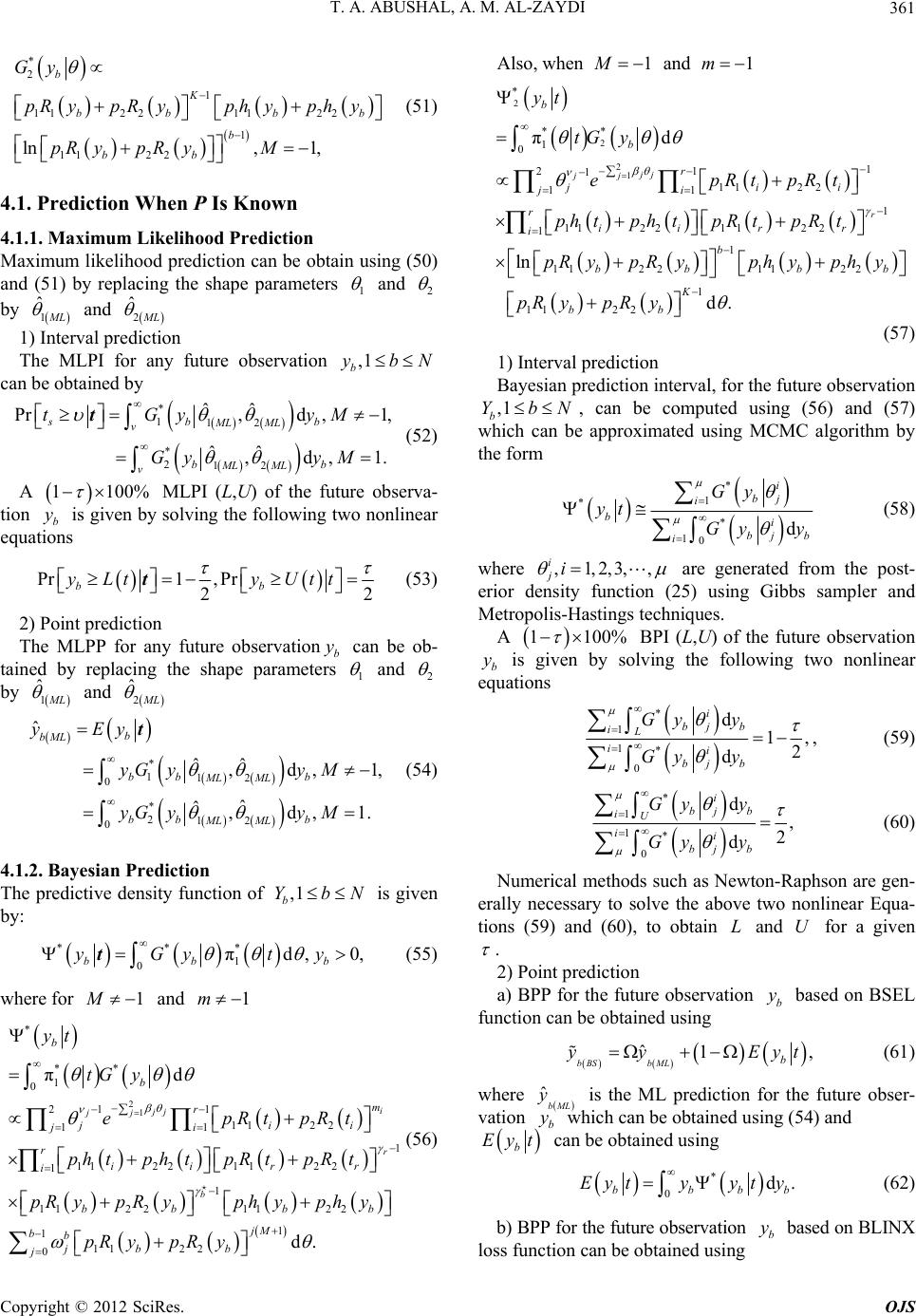
 


T. A. ABUSHAL, A. M. AL-ZAYDI361


 

*
2
1
112211
1
ln ,
b
K
bb
b
Gy
pRypRy ph
pR ypRyM











22
11221,
bb
bb
yphy






ediction When nown
4.
Maximum likelihood prediction in using (50)
by replacing the shparam1
(51)
4.1. PrP Is K
1.1. Maximum Likelihood Prediction
ca
ape
n be obta
eters and (51)

and 2

by

1
ˆ
M
L

and

2
ˆ
M
L

1) Interval prediction
The MLPI for any futu,1
b
ybN re observation


can be obtained by
 

 

*
112
*
212
ˆˆ
Pr ,
ˆˆ
sb
ML ML
v
ML ML
v
tGy
Gy




 



td ,1,
,d,1.
b
bb
yM
yM
 


1100%   MLPI (L,U) of the future observa-
is given by solving the following two nonlinear
(52)
A
tion yb
equations
 
Pr1, PryLt yUt
22
bb
t


he Mr anyutuvatiob can be ob-
t sram1
 t

(53)
2) Point prediction
TLPP fo fre o
hap
bser
e pa
ny
eters ained by replacing the

and 2

by

1
ˆ
M
L
 and

2
ˆ
M
L



 

 

212
,d ,1.
bb
ML ML
yy M 
4.1.2. Baye
*
112
0
*
0
ˆˆ
,d
,1,
ˆˆ
b
bML
bb b
ML ML
b
yG yy M
yG








sian Predi
The predictive dens,1
b
YbN is given
by:
ˆ
yEyt
(54)
ction
ity function of



*
1
πd, 0,
b b
y ty   (55)
**
0
b
yG



t
where for 1
M
 and 1m




  


 

2
1
*
**
1
0
21
1
112 2
11
1
112 21122
1
11 22
1
1122
0
πd
d.
i
jj jj
r
b
b
m
r
jii
ji
r
iir r
i
bb
jbb
tG y
epRtpRt
ph tphtpR tpRt
phyphy











 
1
11 2 2
b
bb
p RypRy

 

1jM
bb
jpR ypR y

yt






 

  









(56)
Also, when 1
M
 and 1m












 
 
   
 
 
2
2
1
*
1
0
1
21
1
112 2
11
1
112 21122
1
1
11 2211 22
1
1122
πd
ln
d.
jj
jj
r
b
r
ji i
ji
r
iir r
i
b
bb b
K
bb
yt
tG y
epRtpRt
ph tphtpR tpRt
pRypRy phyphy
pR ypRy

















 


  
 


b
2
**
b


   



 





(57)
1) Interval prediction
ction ifor the future observation
b
Y

Bayesian predinterval,
,1 bN

, compcan beuted using (56) and (57)
which can be approximated using MCMC algorithm by
the form




*
1
*
*
10d
i
bj
i
bi
bj b
i
Gy
yt Gy y









 (58)
where ,1,2,3,,
i
ji

  are generated from the post-
erior density function (25) using Gibbs sampler and
Metropolis-Hastings techniques.
A


1 100%   BPI (L,U) of the future observation
b
y is given by solving the following two nonl
equatio
inear
ns



*
1
1*
0
d
1,
2
d
i
bj b
iL
ii
bj b
Gy y
Gy y









, (59)




*
1
1*
0
d
,
2
d
i
bjb
iU
ii
bj b
Gy y
Gy y










 (60)
Numerical methods such as Newton-Raphson are gen-
ecessary to solveerally n the above two nonlinear Equa-
tions (59) and (60), to obtain L and U for a given

.
2) Pn
a) BPP for the future observation b y based on BSEL
function ca
oint predictio
n be obtained using
 


ˆ1,
bBS bMLb
yy Eyt
 (61)
where

ˆbML
y is the ML prediction for the future obser-
vation b y which can be obtained using (54) and


b
Eyt can be obtained using
 
*
0d.
bbbb
Eytyyt y


 (62)
b) BPP for the future observation b y based on BLINX
loss function can be obtained using

T. A. ABUSHAL, A. M. AL-ZAYDI 362




ˆ
1ln 1,
bML b
ay
ye Eet



 (63)
bB L
ay



w
ing
a
here

ˆbML y is the ML prediction for the future obser-
vation b y which can be obtained us (54) and

b
ay
Ee t
 can be obtained using


*.d
bb
ay ay
Eeteyty



 (64)
4.2.1. Maximum Likelihood Prediction
Maximum likelihood prediction can be o
and (51) by replacing thete,
0bb
4.2. Prediction When p and θi Are Unknown
btain using (50)
e paramrs p1

and 2

by
 
1
ˆ
,
ˆ
M
LML
p  and

2
ˆ
M
L

1) Interval prediction
The maximum likelihood Interval prediction (MLIP)
for any futu,1
b
ybN can be
by
re observation obtained
 

 

212
1,
ˆd,1.
b ML ML ML
vp yM



va-
ear

*
112
*
ˆˆˆ
Pr,,d ,
ˆˆ
,,
sb b
MLML ML
v
tGy pyM
Gy




 



t
b
(65)
A

1100%   MLPI (L,U) of the future obser
tion b y is given by solving the following two nonlin
equations
 
Pr1, Pr
22
bb
yLtt yUtt


 
 
(6) 6
2) Point prediction
The MLPP for any future observation ,1
b
ybN


can be obtained by replacing the parameters p, 1

and
2

by ˆ , ˆ
 1 
M
LML 2
ˆ
p  and

M
L



 

 

*
112
0
*
212
ˆ
ˆˆˆ
,,
ˆˆ ˆ
,,
bML
ML ML ML
ML ML
v
b
b
bML
y
Gy p
Eyt
y
yG yp








d, 1,
d, 1.
bb
bb
yM
y M


(67)
. B
tive density ,1
b
ybN is given
by:
4.2.2ayesian Prediction
The predicfunction of



1
**
2
*
,πdd ,0
b b
yGyp py  

 tt (68)
00
b

where for 1
M
 and 1m



11
1
***
2
πyGy
00 ,dd.
bb
p p



tt (69)
hen


Also, w 1
M
 and 1m


  
*
2
πdd .p p
22
1
**
00 ,
bb
yGy

 tt (70)
1) Interval prediction
Bayesian prediction interval, for the future observation
,1
b
ybN




, can be computed using (69) and
which can be approximated using MCMC algorithm by
the form
(70)




*,
,
ii
bj
ii
jb
Gyp
dy



 (71)
e ,,1,2,,
ii
j
pi
1
*
i
b
yt





10b iGy
p


wher

are generated from the pos-
terior density function (39) using Gibbs sampler and Me-
tropolis-Hastings techniques.

A

100% 
(L,U) o the future observation
en by the flowing two nonlinear
equations
1 BPI f
b
y is givsolving ol



*
1
1*
0
,d
1,
2
ii
bjb
iL
ii
bjb
Gyp y
G y




,d
i
y
p






 (72) 




*
1,d
,
2
,d
ii
bjb
iU
ii
Gypy
yp y



1* iG
0bj
b




 (73)
Numerical



methods such as Newton-Raphson are nec-
essary to solve the above two nonlinear equations (72)
and (73), to obtain L and U for a given

.
2) Point prediction
a) BPP for the future observation b y ba
function can be obtained using
 
sed on BSEL



1,
Lb
Eyt  (74)
where

ˆbML
y is the ML prediction for the future obser-
vany ich ca
ˆ
bBS bM
yy

bwh tio n be obtained using (67) and


b
yt E
 
0d.
bbbb
Eytyyt y
 (75)
2) BPP for the future observation b y base
loss function can be obtained using


d on BLINX



ˆ
1ln 1
bML
bBL
ay
ye Ee
a


,
b
ay t






 (76)

where

ˆbML
y is the ML prediction for the future obser-
vation b y which can be obtained using (67) and


b
ay
Ee t
 can be obtained using



0d.
bb
ay bb
Ee teyy


 (77)
ayt

5. Simulation Procedure
In this subsection we will consider the upper record val-
ich cues whan be obtained from the GOS by taking
1, 1mk

 and 1
r


. In this section, we will
nt a
com-
pute poind interval predictors of future upper record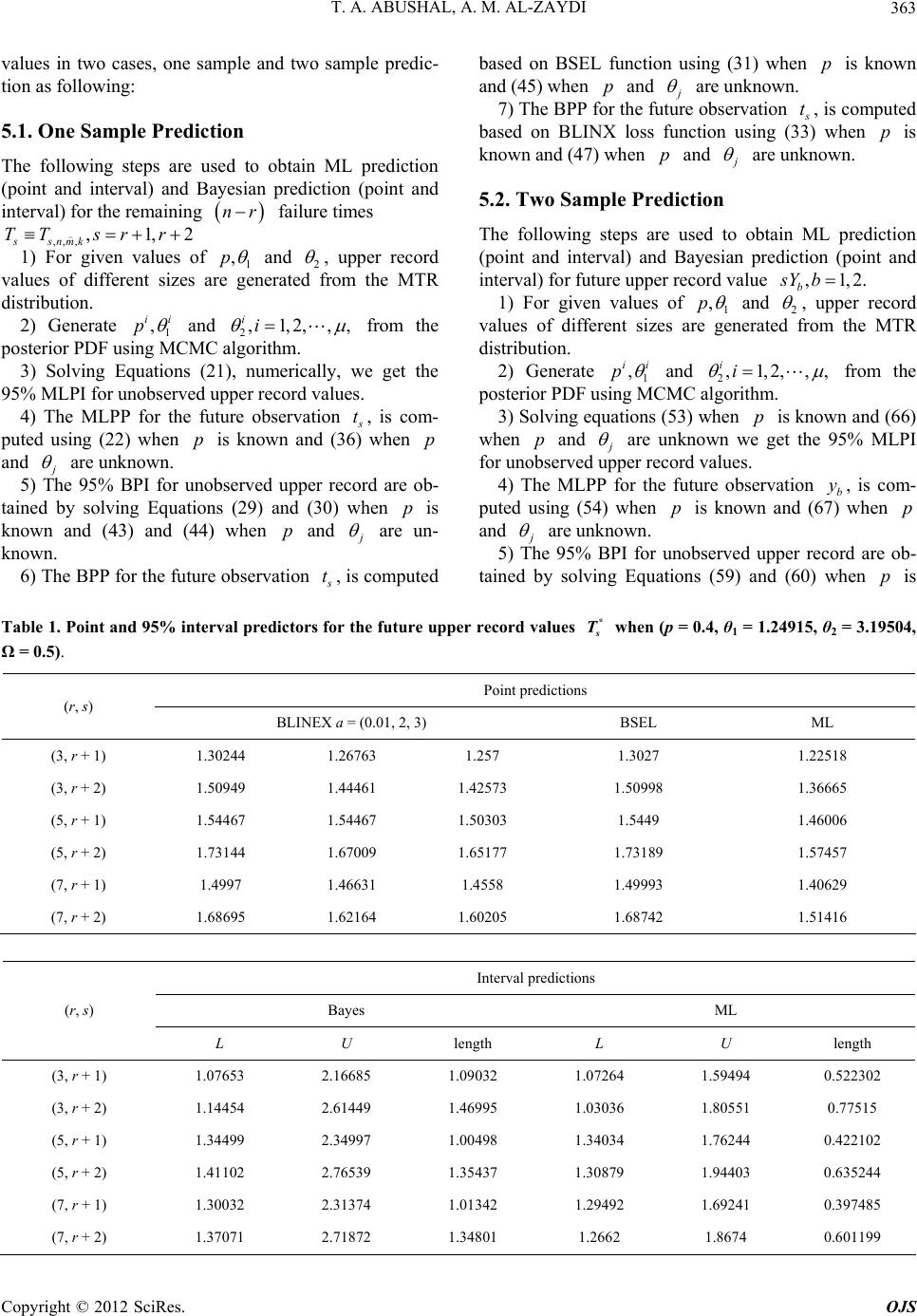

T. A. ABUSHAL, A. M. AL-ZAYDI 363
values in two cases, one sample and two
tion as following:
The fos are used to obtain ML prediction
nd Bayesian prediction (poi
inin

nr
sample predic-
5.1. One Sample Prediction
llowing step
nterval) a
r the rema
(point and i
interval) fo
nt and
g

failure times
,nmk

r
,, 1,2 ss
TTr r
1) Fogiven values of 1 ,p
,s

and 2

, upper record
val rated from the MTR
din.
rate 1
ues of
stributio
2) Gene
different sizes are gene
,
ii
p

and i
2,1,2,,i

  from the 
posterior PDF using MCMC algorithm.
merically, we get the
recordues.
3) Solving Equations (21),
95% MLPI for unobserved uppe
nu
r val
4) The MLPP for the future observation
s
t, is com-
puted using (22) when p is known and (36) when p
and
j

are . unknown
5) The 95% BPI for unobserved upper record are ob-
tained by solving Equations (29) and (30) when p is
known and (43) and (44) when p and
j

are un-
known.
6) The BPP for the future observation
s
t, is computed
based on BSEL function using (31) when p is known
and (45) when p and
j

are unknown.
7) The BPP for the future observation
s
t, is computed
based on BLINX loss function using (33) when p
knowand (47) when pis n and
j

are unknown.
t p
ti
5.2. Two Sample Prediction
The following steps are used to obain MLrediction
(point and interval) and Bayesian predicon (point and
interval) for future upper record value ,1,2.
b
sYb 
1) For given values of 1 ,p

and 2

, upper record
vafrolues of different sizes are generated m the MTR
distribution.
2) Generate 1
,
ii
p

and 2,1,2,,
ii

  fromthe
posterior PDF using MC algthm. CM ori
p is known and (66) 3) Solving equations (53) when
when p and
j

are unknown we get the 95% MLPI
nd (67) whn p
an
for unobserved upper record values.
4) The MLPP for the future observation b y, is com-
puted using (54) when p is known ae
d
j

are unknown.
5) The 95% BPI for unobserved upper record are ob-
tained by solving Equations (59) and (60) when p is
er 915, θ = 3.19504, record values * T when (p = 0.4, θ = 1.24Table 1. Point and 95% interval predictors for the future upp
Ω = 0.5).
s1 2
Point predictions
(r, s)
BLINEX a = (0.01, 2, 3) BSEL ML
(3, r + 1) 1.30244 1.26763 1.1.22518 257 1.3027
(3, r + 2) 1.50949 461 1.441.4257
(5, r + 154467 1.54467 1.5030
+ 1) 1.46631 1.4558 1.49993 1.40629
(7, r + 2) 1.68695 1.62164 1.61.68742 1.51416
3 1.50998 1.36665
3 1.5449 1.46006 ) 1.
(5, r + 2) 1.73144 1.67009 1.65177 1.73189 1.57457
(7, r 1.4997
0205
Interval predictions
Bayes ML (r, s)
L U length L U th leng
(3, r + 1) 1.07653 2.16685 11.07261.59494 302 .09032 4 0.522
(3, r + 2) 1.14454 2.61449 11.03031.80551 515
11.34031.76244 102
(5, r + 2) 1.41102 2.76539 1.7 1.30879 1.94403 0.635244
(7 ) 1.30032 2.31374 1.0192 1.69241 0.397485
(7, r + 2) 1.37071 1.34801 1.2662 1. 0.601199
.46995 6 0.77
(5, r + 1) 1.34499 2.34997 .00498 4 0.422
3543
, r + 1342 1.294
2.71872 8674

T. A. ABUSHAL, A. M. AL-ZAYDI 364
Table 2. Point and 95% interedictors fohe future up values when (p = 0.391789, θ1 = 0.307317, θ2 =
3.33166, 5).
t predictio
rval pr tper record*
s
T
Ω = 0.
Poinns
(r, s)
BLINE 2, 3) EL MX a = (0.01,BSL
(3 7 2.2174, r + 1) 2.322 2.23435 2.21354 2.32287
(3, 2) 2.68054 2.52154 2.48465 2.68226 2.4958
(5, 1) 2.81243 2.74901 2.73223 2.813 2.74014
2.66724 2.62719 2.61879 2.6678 2.62507
(7, r + 2) 2.8745 2.79894 2.72.87574 2.79966
r +
r +
(5, r + 2) 3.13233 3.01438 2.98352 3.13346 3.00112
(7, r + 1)
8385
Interval predictions
Bayes ML (r, s)
L U lL U gth ength len
(3, r + 1) 1.91839 421.91487 2.94288 01 .03255 .11416 1.028
(3, r + 2) 1.80949 53.1.82973.35066 09
412.46333.42614 751
522.53063.82785 24
(7, r + 1) 2.44491 3.71097 1.26605 2.44436 3.08759 0.643231
(7, r + 2) 2.39459 4.67043 2.27746 3.37074 0.97328
.02409 2146 7 1.52
(5, r + 1) 2.46589 .17173 .70584 9 0.962
(5, r + 2) 2.54923 .01563 .46641 1 1.297
584 2.39
Table 3. Point and 95% interval predictors foe future upprd values Y b = 1, 2 when ( 0.4, θ1 = 1.22 =
3.1950 5).
int predictio
r ther reco*
b, p =4915, θ
4, Ω = 0.
Pons
(r, b)
B0.01, 2, BSELINEX a = (3) L ML
(3.1) 0.669076 0084 0.552831 0.6690.58789 0.55108
(3.2) 1.06708 0272 0.901294 1.068
9 1745 0.554524 0.6680.
(5.2) 1.05059 0.926826 0.888678 1.05157 0.879144
(7.2) 0.999761 0.874356 0.838862 1.00077 0.790802
0.9414 0.905675
(5.1) 0.667370.58033 557414
(7.1) 0.637403 0.552511 0.526817 0.638057 0.506104
Interval predictions
BayL es M
(r, b)
L Ulength (CP L ) ) Ulength (CP
(3.1) 0.2.031.91158 (96.0.0850494 166 1. 123947 553 16) 1.4738661 (97.70)
(3.2) 0.2.702.32429 (94.0.267226 068 1.
0.1.971.85479 (95.0.0926795 062 1.
0.2.582.20882 (94.0.289275 782 1.
(7.1) 0.122419 1.93781 1.81539 (96.01) 0.0854495 1.20807 1.12263 (95.03)
0.376222 2.51787 2.14165284 1.55638 1.2901 (95.43)
37762 191 97) 1.963957 (98.54)
(5.1) 122991 778 90) 1.3626794 (96.50)
(5.2) 377125 594 75) 1.7546854 (97.63)
(7.2) (94.49) 0.266

T. A. ABUSHAL, A. M. AL-ZAYDI 365
Table 4. Point and 95% interval predictors future upper record values *
b
Y, b = 1, 2 when (.391789, θ1 = 0.307317,
θ2 = 3.33166, Ω = 0.5).
predi
for thep = 0
Pointctions
(r, b)
a =(0.BSEL BLINEX 01, 2, 3) ML
(3.1) 869 696151 63902 0.878460.8760.0.2 0.827878
(3.2) 559 22759 09298 1.5681
) 0.1 707462 647328 0.889363
) 375 25773 12298 1.5657
(7.2) 1.44473 1.15656 1.04976 1.44702 1.26946
1.561.1.1 1.47625
(5.188790.0.0.828237
(5.21.561.1.9 1.46954
(7.1) 0.813281 0.645203 0.598027 0.814804 0.695196
Interval predictions
Bayes ML (r
L U length (CP) L U )
, b)
length (CP
(30.10032.95917 8588 (97.15357 1 5.56) .1) 72 2.) 0.09742.48912.39167 (9
(30.32003.97264 65263 (97.32)313335 5 36)
(50.09812.80057 5 (96.91446 4 5.42)
(50.31903.64706 32801 (97.66)297965 2 16)
(7.1) 0.0971018 2.83087 2.73377 (96.94) 0.0826299 2.22201 2.13938 (94.13)
(7.2) 0.304841 3.74134 3.4365 (343 2.87667 2.61324 (93.33)
.2) 05 3. 0.3.18482.87151 (95.
.1) 198 2.7024) 0.09152.42922.33769 (9
.2) 49 3. 0.3.08572.78776 (95.
97.94) 0.26
known and (72) and73) wh p and (en
j

are un-
known.
6) TPP for theeris co
puted b onLusi p
know 4)
he B future obs
1)
vatio
Point and 95% interval pr for futr-
ns are obned using a onsample anle
es b MTR ion. e
lized record v
is evm all tabat, the lengthe
nd BPI as thle size increase.
r fiple size lengthI
PI inincreasi
edictors
e-
ure obse
d two-samptai
schem ased on adistributOur results ar
specia to upperalues.
2) It
MLPI a
ident fro
decrease
les th
e samp
s of th
3) Foxed samr the s of the MLP
and Bcrease by ng
s
o
vati
ng (
on b y, m-
ased61) when is BSE
when
function
n and (7p and
j

arunk
7) TPP for thervatis co
puted bon BLon usihen
is know6)
e nown.
ion y, he Be future obsb
ng (63) w
m-
ased INX
whe
loss functi p
n and (7n p and
j

arn.
8) Ge 10, 000 sameach of size 6 from
TR dtion, then calcue covercentag
w m
n,
e unknow
nerate
istribu
ples
late th
N =
rage pe
a
e
r b.
The pee coveraves be
number of observed values.
CES
ps, “A Concep
4) rcentagge improy use of a larg
M
(CP) of b Y.
The computational (our) results ere coputed by
using Mathematica 7.0. When p is know the prior
parameters chosen as 12 1 2
2.3, 2.7,0.5, 1.3




which yield the generated values of 11.24915

and
23.19504

. While, in the case of four parameters are
unknown the prior parameters

1212 1 2
,,,,, bbcc dd cho-
sen as

1.2,2.3, 2, 2,0.3,3 which yield the generat
va
REFEREN
[1] U. Kamt of Generalized Order Statistics,”
Journal of Statistical Planning and Inference, Vol. 48,
No. 1, 1995, pp. 1-23.
doi:10.1016/0378-3758(94)00147-N
[2] M. Ahsanullah, “Generalized Order Statistics from Two
rm Distribution,” Communications in Sta-
nd Methods, Vol. 25, No. 10, 1996, pp.
.1080/03610929608831840
ed
Parameter Unifo
tistics—Theory a
lues of 0.391789p, 12
0.307317, 3.33166



.
In Tables 1-4 point and 95% interval predictors for the
future upper record value are computed in case of the
on
2311-2318. doi:10
[3] M. Ahsanullah, “Generalized Order Statistics from Expo-
nential Distributiuon,” Journal of Statistical Planning and
Inference, Vol. 85, No. 1-2, 2000, pp. 85-91.
doi:10.1016/S0378-3758(99)00068-3
[4] U. Kamps and U. Gather, “Cha
e- and two sample predictions, respectively.
5.3. Conclusions
It may be observed: racteristic Property of

T. A. ABUSHAL, A. M. AL-ZAYDI 366
el for
378-3758(00)00074-4
Generalized Order Statistics for Exponential Distribu-
tions,” Applicationes Mathematicae (Warsaw), Vol. 24,
No. 4, 1997, pp. 383-391.
[5] E. Cramer and U. Kamps, “RationsExpectations of
Functions of Generalized Order Statistics,” Journal of
Statistical Planning and Inference, Vol. 89, No. 1-2, 2000,
pp. 79-89. doi:10.1016/S0
[6] M. Habibullah and M. Ahsanullah, “Estimation of Pa-
rameters of a eneralized Order
statistics,” Comand Me-
Pareto Distribution by G
munications in Statistics—Theory
thods, Vol. 29, No. 7, 2000, pp. 1597-1609.
doi:10.1080/03610920008832567
[7] Z. F. Jaheen, “On Bayesian Prediction o
Order Statistics,” Journal of Statisticf General al Theory and Ap-
2005, pp.
ized
plications, Vol. 1, No. 3, 2002, pp.191-204.
[8] Z. F. Jaheen, “Estimation Based on Generalized Order
Statistics from the Burr Model,” Communications in Sta-
tistics—Theory and Methods, Vol. 34, No. 4,
785-794. doi:10.1081/STA-200054408
[9] E. K. Al-Hussaini and A. A. Ahmad, “On Bayesian Pre-
dictive Distributions of Generalized Order
Metrika, Vol. 57, No. 2, 2003, pp. 165
Statisti
-176.
cs,”
doi:10.1007/s001840200207
[10] E. K. Al-Hussaini, “Generalized Order Statistics: Prospec-
tive and Applications,” Journal of Applied Statistical Sci-
ence, Vol. 13, No. 1, 2004, pp. 59-85.
s Distribu-
ory and Applications,
oubly Trun-
ents of General-
[11] A. A. Ahmad and T. A. Abu-Shal, “Recurrence Relations
for Moment Generating Functions of Nonadjacent Gen-
eralized Order Statistics Based on a Class of Doubly
Truncated Distributions,” Journal of Statistical Theory
and Applications, Vol. 6, No. 2, 2007, pp. 174-189.
[12] A. A. Ahmad and T. A. Abu-Shal, “Recurrence Relations
for Moment Generating Functions of Generalized Order
Statistics from Doubly Truncated Continuou
tions,” Journal of Statistical The
Vol. 6, No. 2, 2008, pp. 243-257.
[13] A. A. Ahmad, “Relations for Single and Product Mo-
ments of Generalized Order Statistics from D
cated Burr type XII Distribution,” Journal of the Egyp-
tian Mathematical Society, Vol. 15, No. 1, 2007, pp. 117-
128.
[14] A. A. Ahmad, “Single and Product Mom
ized Order Statistics from Linear Exponential Distribu-
tion,” Communications in Statistics—Theory and Methods,
Vol. 37, No. 8, 2008, pp. 1162-1172.
doi:10.1080/03610920701713344
[15] Z. A. Aboeleneen, “Inference for Weibull Distribution
under Generalized Order Statistics,” Mathematics and
Computers in Simulation, Vol. 81, No. 1, 2010, pp. 26-36.
doi:10.1016/j.matcom.2010.06.013
[16] S. Abu El Fotouh, “Estimation for the Parameters of the
Weibull Extension Model Based on Generalized Order
Statistics,” International Journal of Contemporary Mathe-
matical Sciencess, Vol. 6, No. 36, 2011, pp. 1749-1760.
[17] S. F. Ateya, “Prediction under Generalized Exponential
Distribution Using MCMC Algorithm,” International Ma-
thematical Forum, Vol. 6, No. 63, 2011, pp. 3111-3119.
[18] S. F. Ateya and A. A. Ahmad, “Inferences Based on Gen-
eralized Order Statistics under Truncated Type I Gener-
alized Logistic Distribution,” Statistics, Vol. 45, No. 4,
2011, pp. 389-402. doi:10.1080/02331881003650149
[19] B. S. Everitt and D. J. Hand, “Finite Mixture Distribu-
tions,” Cambridge University Press, Cambridge, 1981.
[20] D. M. Titterington, A. F. M. Smith and U. E. Makov, “Sta-
titute of Statistical
pp. 261-265.
tistical Analysis of Finite Mixture Distributions,” John
Wiley and Sons, New York, 1985.
[21] K. E. Ahmad, “Identifiability of Finite Mixtures Using a
New Transform,” Annals of the Ins
Mathematics, Vol. 40, No. 2, 1988,
doi:10.1007/BF00052342
[22] G. J. McLachlan and K. E. Basford, “Mixture Models:
Inferences and Applications to Clustering,” Marcel Dek-
ker, New York, 1988.
[23] Z. F. Jaheen, “On Record Statistics from a Mixture of
Two Exponential Distributions,” Journal of Statistical
Computation and Simulation, Vol. 75, No. 1, 2005, pp. 1-
11. doi:10.1080/00949650410001646924
[24] K. E. Ahmad, Z. F. Jaheen and Heba S. Mohammed,
“Bayesian Prediction Based on Type-I Censored Data
from a Mixture of Burr Type XII Distribution and Its Re-
ciprocal,” Statistics, Vol. 1, No. 1, 2011, pp. 1-11.
doi:10.1080/02331888.2011.555550
[25] E. K. AL-Hussaini and M. Hussein, “Estimation under a
Finite Mixture of Exponentiated Exponential Components
Model and Balanced Square Error Loss,” Open Journal
of Statistics, Vol. 2, No. 1, 2012, pp. 28-38.
doi:10.4236/ojs.2012.21004
[26] M. A. M. Ali-Mousa, “Bayesian Prediction Based on Pareto
Doubly Censored Data,” Statistics, Vol. 37, No. 1, 2003,
pp. 65-72. doi:10.1080/0233188021000004639
[27] A. S. Papadapoulos and W. J. Padgett, “On Bayes Esti-
mation for Mixtures of Two Exponential-Life-Distribu-
tions from Right-Censored Samples,” IEEE Transactions
on Reliability, Vol. 35, No. 1, 1986, pp. 102-105.
doi:10.1109/TR.1986.4335364
[28] A. F. Attia, “On Estimation for Mixtures of 2 Rayleigh
Distribution with Censoring,” Microelectronics Reliabil-
ity, Vol. 33, No. 6, 1993, pp. 859-867.
doi:10.1016/0026-2714(93)90259-2
[29] K. E. Ahmad, H. M. Moustafa and A. M. Abd-El-Rah-
man, “Approximate Bayes Estimation for Mixtures of Two
Weibull Distributions under Type II Censoring,” Journal
of Statistical Computation and Simulation, Vol. 58, No. 3,
1997, pp. 269-285. doi:10.1080/00949659708811835
[30] A. A. Soliman, “Estimators for the Finite Mixture of
Rayleigh Model Based on Progressively Censored Data,”
Communications in Statistics—Theory and Methods, Vol.
35, No. 5, 2006, pp. 803-820.
doi:10.1080/03610920500501379
[31] M. Saleem and M. Aslam, “Bayesian Analysis of the
Two Component Mixture of the Rayleigh Distribution
Assuming the Uniform and the Jeffreys Priors,” Journal
of Applied Statistical Science, Vol. 16, No. 4, 2008, pp.
105-113.

T. A. ABUSHAL, A. M. AL-ZAYDI 367
Properties of the Bayes
sian Estimation Us-
saini and K. E. Ahmad, “On the Identifiabil- [32] M. Saleem and M. Aslam, “On Prior Selection for the
Mixture of Rayleigh Distribution Using Predictive Inter-
vals,” Pakistan Journal of Statistics, Vol. 24, No. 1, 2007,
pp. 21-35.
[33] M. Saleem and M. Irfan, “On
ity o
estimates of the Rayleigh Mixture Parameters: A Simula-
tion Study,” Pakistan Journal of Statistics, Vol. 26, No. 3,
2010, pp. 547-555.
[34] A. Zellner, “Bayesian and Non-Baye
ing Balanced Loss Functions,” In: J. O. Berger and S. S.
Gupta, Eds., Statistical Decision Theory and Methods. V,
Springer, New York, 1994, pp. 339-390.
[35] M. J. Jozani, E. Marchand and A. Parsian, “Bayes Esti-
mation under a General Class of Balanced Loss Func-
tions,” Universite de Sherbrooke, Sherbrooke, 2006.
[36] E. K. Al-Hus
f Finite Mixtures of Distributions,” IEEE Transac-
tions on Information Theory, Vol. 27, No. 5, 1981, pp.
664-668. doi:10.1109/TIT.1981.1056389
[37] K. E. Ahmad and E. K. Al-Hussaini, “Remarks on the
Non-Identifiability of Mixtures of Distributions,” Annals
of the Institute of Statistical Mathematics, Vol. 34, No. 1,
1982, pp. 543-544. doi:10.1007/BF02481052
[38] S. J. Press, “Subjective and Objective Bayesian Statistics:
tion
Principles, Models and Applications,” Wiley, New York,
2003.
[39] J. Aitchison and I.R. Dunsmore, “Statistical Predic
Analysis,” Cambridge University Press, Cambridge, 1975.