Journal of Minerals & Materials Characterization & Engineering, Vol. 9, No.2, pp.89-103, 2010
jmmce.org Printed in the USA. All rights reserved
89
Coag-Flocculation Kinetics and Functional Parameters Response of Mucuna
Seed Coagulant to pH Variation in Organic Rich Coal Effluent Medium
M.C. Menkiti1*, P.C. Nnaji2, C.I. Nwoye3, O.D. Onukwuli1
1Department of Chemical Engineering, Nnamdi Azikiwe University, Awka, Nigeria.
2Enugu State Water Corporation, Enugu, Nigeria
3Department of Metallurgical and Materials Engineering, Federal university of Technology
Owerri, Nigeria
*Corresponding author:
ABSTRACT
The coag-flocculation performance of Mucuna Seed Coagulant as affected by pH variation in
coal washery effluent has been investigated at room temperature using various dosages of
unblended Mucuna Seed Coagulant. In addition, coag-flocculation parameters such as Coag-
flocculation reaction order α, αth order coag-flocculation constant K, Collision factor for
Brownian Transport βBr, Smoluchowski constant KR,, Collision Efficiency εp, and Coagulation
Period τ1/2 were determined. Turbidity measurement was employed using the nephelometric
(turbidimetric) standard method while Mucuna Seed Coagulant preparation was adopted from
the works of Adebowale and Adebowale (2007). The maximum Mucuna Seed Coagulant
parameter performance is recorded at α of 2, K of 8.3334 x 10-3 m3/kg.s, dosages of (0.15 kg/m3;
0.2 kg/m3; 0.25 kg/m3); pH of 6 and τ1/2 of 1.7339 sec while the minimum parametric
performance is recorded at α of 1; K of 6.3001 x 10-4 s-1; dosage of 0.2kg/m3; pH of 8 and τ1/2 of
1100.2161seconds. The minimum value of coag-flocculation efficiency E (%) recorded is greater
than 88.00 %. Conclusively; Mucuna Seed Coagulant is an effective coagulant obeying the
theory of fast coagulation at the conditions of the experiment.
Keywords: Coag-flocculation, Kinetics, Coal effluent, Mucuna, Coagulation
1. INTRODUCTION
1.1 Background
Coag-flocculation is a core purification process, which finds wide range of application in water
and waste water treatment facilities. Conceptually, Coag-flocculation is the process of adding
substances to aqueous effluent to make suspended particles to bind together (coagulate) and
subsequently aggregating into visible flocs (flocculation) that settle out of the water. This is
achieved when the stabilized particles are aided to overcome their repulsive forces to form blobs
of flocs [1, 2, 3, 4]. Among the factors that affect the process are raw effluent quality,
temperature, pH, etc [5].
In particular, coag-flocculation in conjunction with other treatment processes is regarded as a
viable option for the treatment of aqueous effluent such as coal washery effluent. Coag-
flocculation can be achieved by any of the common coagulants such as alum, lime etc. The

90 M.C. Menkiti, P.C. Nnaji, C.I. Nwoye, O.D. Onukwuli Vol.9, No.2
Coag-flocculation behaviors of these common compounds have been well investigated with little
or no attention given to the Coag-flocculation potentials of bio derivatives. To this end, a focus is
hereby given to the study on Mucuna bean seed (MBS) as a potential source of Coag-
flocculation derivative. Mucuna sloanei is an annual twinning tropical plant with pods containing
seed bean, which is the bearer of the active components (proteins) that is processed into Mucuna
Seed Coagulant (MSC). The seeds are high in proteins (20-30%), lipids, fibers, minerals and L-
dopa [6]. MSC is a non-toxic, biodegradable and biocompatible compound.
Against this backdrop, this work endeavors to explore and generate interest in the utilization of
MBS as a coagulant. Also investigated are Coag-flocculation performance and kinetics of MSC
under various pH of coal washery effluent, a typical medium for this kind of study. Thus, if well
developed, MSC takes on a significant importance towards finding alternative replacement for
the chemical coagulants/flocculants.
1.2 Theoretical Principles and Model Development
For a uniformly composed coag-flocculation phase with negligible influence of external forces:
=
⎥
⎦
⎤
⎢
⎣
⎡
∂
∂
==
nTP
i
ii n
G
G
,,
μ a constant ….1
Thus0=
i
d
μ
….2
For each of the species i present [7].
G is the total Gibbs free energy
ni is the number of moles of component i
For dilute solutions
i
o
ii CRT ln+≈
μμ ….3
A shift from the equilibrium generates diffusional process represented by:
dx
d
fd
μ
−= ….4
Recall N
R
KB= such that for single N , KB=R
Hence iB
o
ii CTK ln+≈
μμ …..5
Where KB is Boltzmann constant; i
μ
is chemical potential
R is universal gas constant; Ci is concentration
N is Avogadro’s constant; x is diffusion distance
Combining equations 4 and 5 yield:
()
iBid CTK
dx
d
fln
0+−=
μ …..6
dx
dC
C
K
fi
i
B
d−= …7
The viscous drag force on the particles due to surrounding fluid is:
dd BUf = ….8
And di CUJ = ….9
Where B is friction factor
Ud is terminal diffusing velocity
Ji is flux of diffusing material
fd is drag force
From Fick’s law
(
)
dx
dc
JD −=
′ …10
Where D′ is diffusion coefficient

Vol.9, No.2 Coag-flocculation Kinetics and Functional Parameters 91
Combining equations 8, 9 and 10 yield
()
dx
dc
c
B
f
Dd
−
=
′ …11
Comparing equations 7 and 11 generate Einstein’s equation:
B
TK
DB =
′ …12
For similar phase, the rate of successful collisions between particles of sizes i and j to form
particle of size K is [8, 5]:
Nij = εp β (i,j) ninj …13
where Nij is the rate of collisions between particles of size i and j(mass concentration / time)
εp is collision efficiency
β(i,j) is collision factor between particles of size i and j
ninj is particle concentration for particles of size i and j, respectively.
Assuming monodisperse, no break up and bi particle collision, the general model for perikinetic
coag-flocculation is given as [9, 5]
ki
i
ji
kji
knnkinnji
dt
dn ∑∑ ∞
==+
−=
1
),(),(
2
1
ββ …14
where dt
dnk is the rate of change of concentration of particle of size K (concentration / time).
β
is a function of the coag-flocculation transport mechanism .The appropriate value of
β
for
Brownian transport is given by [10]:
η
εβ
TkB
pBR 3
8
= …15
Where B
k is Boltzmann’s constant (J/K)
T
is Absolute temperature (K)
The generic aggregation rate of particles (during coagulation / flocculation) can be derived by the
combination of equations 2 and 3 to yield:
α
t
tKN
dt
dN =− …16
Where t
N is total particle concentration at timet,
∑
=kt nN (mass / volume)
K is the th α order coag-floculation constant
α is the order of coag-floculation process
And BR K β
2
1
= …17
Where BR
β
is collision factor for Brownian transport
Also, RpBR K
ε
β
= …18
Combining equations 4, 5 and 6 produce:
=− dt
dNt
α
β
tBR N
2
1 ….19
α
ε
tRpNK.
2
1
= …20
Where R K is the Von smoluchowski rate constant for rapid coagulation [10]
However DRK R′ =
π
8 ….21
aRp2= ….22
Where D′ is particle diffusion coefficient
a is particle radius.
From Einstein’s equation:B
T
KD B
=
1 .…23

92 M.C. Menkiti, P.C. Nnaji, C.I. Nwoye, O.D. Onukwuli Vol.9, No.2
From Stroke’s equation:aB
πη
6= ….24
where B is the friction factor
η is the viscosity of the fluid
combining equations 21 to 24 gives:
α
η
ε
t
B
p
tN
TK
dt
dN
3
4
=− .…25
Comparing equations16 and 25 show:
η
ε
TK
KB
p
3
4
= ....26
For perikinetic aggregation,
α
theoretically equals 2 as would shown below [12, 7]:
From Fick’s law,
dR
dN
RDJt
pf
2
4 π
′
= ..27
Integrating equation 27 at initial conditions0
=
t
N,aR 2
=
:
∫∫ =
′
pt
RN
Nt
p
pf dN
R
dR
D
J
020
4 π
...28
Therefore 0 8aNDJf′ =
π
…29
0
2
1NKR⋅⋅= ...30
For central particle of same size undergoing Brownian motion, the initial rate of rapid coag-
flocculation is:
0 NJ
dt
dN
pf
t⋅⋅=−
ε …31
2
0
2
1NK pR ⋅⋅⋅=
ε
2
0
3
4N
TKB
p⋅=
η
ε ...32
2
3
4
t
B
pN
TK
η
ε ≡ at 0>t
Hence, from equation 32,2=
α
However in real practice, empirical evidence shows that in general21 ≤
≤
α
[13,14].Based on
this , what is required to evaluate K is to determine the line of better fit between
=
α
1 and 2
while the experimental data are fitted into linearised form of equation 16.
Hence, for1=
α
, equivalence of equation 16 yields:
−=
dt
dN KN ...33
Integrating within the limits produces
Kdt
N
dN
N
N
t
∫∫
−=
00 ...34
Hence
)
(
0
ln
1
ln NKt
N−= ...35
Plot of
)
(
N
1
ln vs.t gives a slope of K and intercept of)ln( 0 N
−
.
For2=
α
; equivalence of equation 16 yields:
2 KN
dt
dN −= …36
Hence:

Vol.9, No.2 Coag-flocculation Kinetics and Functional Parameters 93
∫∫ −=tN
NdtK
N
dN
0
2
0
…37
0
1
1
N
Kt
N+= ...38
Plot of ln
)
(
N
1 Vs t produces a slope of K and intercept of
0
1N.
For the evaluation of coagulation period (21
τ
), from Equation 38:
KtN
N
N
0
0
1+
= ....39
⎥
⎥
⎥
⎥
⎦
⎤
⎢
⎢
⎢
⎢
⎣
⎡
⎟
⎠
⎞
⎜
⎝
⎛
+
=
KN
t
N
0
0
1
1
...40
Where ⎥
⎦
⎤
⎢
⎣
⎡
=KN0
1
τ
Hence:
() τ /1
0
t
N
N+ = …41
When
τ
=t, equation 41becomes
2
0
N
N= …42
Therefore as 2100 ;5.0
τ
τ
→→ NN
Hence
() KN0
21 5.0
1
= τ for 2nd order ...43
And K
2ln
2
1=
τ for1storder …44
For Brownian aggregation at early stages (t≤30 minutes), equation 14 can be solved
exactly, resulting in the expression [15]:
1
0
1
0
0
)(
1
2
1
1
2
+
−
⎥
⎥
⎥
⎥
⎥
⎦
⎤
⎢
⎢
⎢
⎢
⎢
⎣
⎡
⎜
⎜
⎝
⎛
⎟
⎟
⎠
⎞
+
⎢
⎢
⎣
⎡
⎥
⎥
⎦
⎤
⎟
⎟
⎠
⎞
⎜
⎜
⎝
⎛
=m
m
tm
KN
t
KN
t
N
N ….45
and
[]
[]
1
1
0
)(
1+
−
′
+
′
=m
m
tm
t
t
N
N
τ
τ
...46
Equation 46 gives a generic expression for particle of m-th order .Hence,
For singlets (m=1)
()
⎥
⎥
⎥
⎦
⎤
⎢
⎢
⎢
⎣
⎡
′
+
=2
01
1
1
τ
t
NN ...47
For doublets (m=2)
()
()
⎥
⎥
⎥
⎦
⎤
⎢
⎢
⎢
⎣
⎡
′
+
′
=3
02
1
τ
τ
t
t
NN ….48

94 M.C. Menkiti, P.C. Nnaji, C.I. Nwoye, O.D. Onukwuli Vol.9, No.2
For triplets (m=3)
()
()
⎥
⎥
⎥
⎦
⎤
⎢
⎢
⎢
⎣
⎡
′
+
′
=4
2
03
1
τ
τ
t
t
NN ….49
2. METHODS
The sample of Mucuna bean seed was sourced from Eke central market, Awka Nigeria and
processed to MSC based on the work reported by Adebowale and Adebowale [16].
The jar test was conducted based on standard Bench scale Nephelometric method (single angle
procedure) for the examination pf water and waste water [13,17] using model WZS-185 MC
Turbidimeter, APPNo 688644A Gulenhamp magnetic stirrer and mettler Toledo Delta 320 pH
meter.
3. RESULTS AND DISCUSSION
3.1 Coag-Flocculation Parameters
The values of coag-flocculation functional parameters are presented in tables 1 to 5. The general
trends indicate that for pH of 8 and 10 the values of α = 1 while that of pH of 2 to 6, the α = 2.
The significant of this is that the optimum pH = 6 and this is recorded for α = 2. For the case of α
= 1, it is a shift from theoretical expectation but in line with empirical evidence[13].
The optimum K are recorded for pH=6 for all the dosages, though the coag-flocculation
performance at pH=2 and 4 are very high. These facts are confirmed by the values of τ1/2
recorded between pH=2 and pH=6 with pH of 6 having the lowest values
Generally, the value of α affects that of K inversely. Since K is rate per concentration and K is
associated with energy barrier (KT), it is understandable that for higher α to be obtained, a lower
K is a necessary condition for such phenomenon [12]. The values of K are computed from graphs
represented by selected sample plots of Figs 1 and 2. K (= 0.5βBr) values are les sensitive to
pH=2 to pH=6 for all the dosages studied. Variation in KR is generally minimal as presented in
tables 1 to 5. This is because KR=fn (T, η) both of which did not vary considerably during the
study. The values of α and K are to a large extent consistent with previous works [11].
At nearly invariant values of KR ,εp directly relates to 2K=βBr. The consequence is that high εp
results in high kinetic energy to overcome the zeta potential Zp. The implication is that the
double layer is either reduced or the colloids destabilized to actualize low τ1/2 in favor of
coagulation rate. The results show that high values of τ1/2 corresponds to low εp and K, an
indication of repulsion in the system. τ1/2 values lie within the range of previous works where
milliseconds had been obtained [7].
Generally, the discrepancies in the parameters
(
)
c
pR SPKK 0
)(,,,, εα
can be explained by the
unattainable assumption that mixing of particles and coagulants throughout the dispersion is
100% efficient before any aggregation occurs. The effect of these limitations will be local
increase in particle ratios during the mixing phase given uneven distribution of
particles/coagulant complexes. This complexity makes it impossible to have all α=2 [18].
Another account is the effects of interplay between and among the van der walls forces,
hydrodynamic interactions, type of counter ion and other short range forces which systematically
increase or reduce the values of parameters [15, 19].

Vol.9, No.2 Coag-flocculation Kinetics and Functional Parameters 95
Table 1. Coag-flocculation Functional parameters for varying pH and constant dosage of 0.05
kg/m3 MSC
Parameter pH=2 pH=4 pH=6 pH=8 pH=10
α
2 2 2 1 1
2
R
0.862 0.852 0.945 0.954 0.861
K
3.333x10-
3m3/kg.s
3.333x10-
3m3/kg.s
6.667x10-
3m3/kg.s 7.767x10-4s-1 6.817x10-4s-1
Br
β
6.666x10-
3m3/kg.s
6.666x10-
3m3/kg.s
1.333x10-
2m3/kg.s 1.553x10-3s-1 1.363x10-3s-1
R
K 1.434x10-
17m3/s
1.407x10-
17m3/s
1.549x10-
17m3/s
1.391x10-
17m3/s
1.361x10-
17m3/s
p
ε
4.648x1014kg-1 4.736x1014kg-1 8.607x1014kg-1 11.165x1013m-3 10.019x1013m-3
(sec)
2
1
τ
4.344 4.344 2.167 892.449 1016.820
()
c
SP 0 0.588kg/m3 2.000kg/m3 0.073kg/m3 15.027kg/m3 9.433kg/m3
r
− 3.333x10-3 c2 3.333x10-3 c2 6.667x10-3 c2 7.767x10-4 c 6.817x10-4 c
Table 2. Coag-flocculation Functional parameters for varying pH and constant dosage of
0.1kg/m3 MSC
Parameter pH=2 pH=4 pH=6 pH=8 pH=10
α
2 2 2 1 1
2
R
0.955 0.962 0.992 0.988 0.910
K
5.000x10-
3m3/kg.s
3.333x10-
3m3/kg.s
6.667x10-
3m3/kg.s 7.200x10-4s-1 8.300x10-4s-1
Br
β
10.000x10-
3m3/kg.s
6.666x10-
3m3/kg.s
13.333x10-
3m3/kg.s 1.440x10-3s-1 1.660x10-3s-1
R
K 1.769x10-
17m3/s 1.720x10-17m3/s 1.739x10-17m3/s 1.481x10-17m3/s 1.417x10-17m3/s
p
ε
5.653x1014kg-
1 3.875x1014kg-1 7.668x1014kg-1 9.722x1013m-3 11.712x1013m-3
(sec)
2
1
τ
2.890 4.335 2.167 962.691 835.107
()
c
SP 0 0.625kg/m3 1.666kg/m3 0.833kg/m3 9.853kg/m3 6.424kg/m3
r
− 5.000x10-3 c2 3.333 c2 6.667 c2 7.200x10-4 c 8.300x10-4 c
Table 3. Coag-flocculation Functional parameters for varying pH and constant dosage of
0.15kg/m3 MSC
Parameter pH=2 pH=4 pH=6 pH=8 pH=10
α
2 2 2 1 1
2
R
0.995 0.999 0.830 0.730 0.954
K
3.333x10-
3m3/kg.s
6.667x10-
3m3/kg.s
8.333x10-
3m3/kg.s 2.205x10-4s-1 7.150x10-4s-1
Br
β
6.667x10-
3m3/kg.s
13.333x10-
3m3/kg.s
16.667x10-
3m3/kg.s 4.410x10-3s-1 1.430x10-3s-1
R
K 1.418x10-
17m3/s 1.384x10-17m3/s 1.379x10- 17m3/s
1.284x10-
17m3/s
1.131x10-
17m3/s
p
ε
4.702x1014kg-1 9.631x1014kg-1 12.087x1014kg-
1 3.435x1014m-3 2.528x1014m-3
(sec)
2
1
τ
4.344 2.167 1.734 314.352 969.423
()
c
SP 0 0.500kg/m3 3.333kg/m3 0.0943kg/m3 36.753kg/m3 13.220kg/m3
r
− 3.333x10-3 c2 6.667x10-3 c2 8.333x10-3 c2 2.205x10-3 c 8.300x10-4 c

96 M.C. Menkiti, P.C. Nnaji, C.I. Nwoye, O.D. Onukwuli Vol.9, No.2
Table 4. Coag-flocculation Functional parameters for varying pH and constant dosage of
0.20kg/m3 MSC
Parameter pH=2 pH=4 pH=6 pH=8 pH=10
α
2 2 2 1 1
2
R
0.919 0.8537 0.814 0.975 0.986
K
8.333x10-
3m3/kg.s
5.000x10-
3m3/kg.s
8.333x10-
3m3/kg.s 6.300x10-4s-1 7.550x10-4s-1
Br
β
16.667x10-
3m3/kg.s
10.000x10-
3m3/kg.s
16.667x10-
3m3/kg.s 1.260x10-3s-1 1.510x10-3s-1
R
K 1.418x10-
17m3/s 1.384x10-17m3/s 1.379x10- 17m3/s
1.284x10-
17m3/s
1.425x10-
17m3/s
p
ε
11.757x1014kg
-1 7.223x1014kg-1 12.087x1014kg- 1 9.816x1013m-3 10.592x1013m-3
(sec)
2
1
τ
1.734 2.890 1.734 1100.216 918.076
()
c
SP 0 0.333 kg/m3 0.909 kg/m3 0.1052 kg/m3 4.991 kg/m3 14.869 kg/m3
r
− 8.333x10-3 c2 5.000x10-3 c2 8.333x10-3 c2 6.300x10-4 c 7.550x10-4 c
Table 5. Coag-flocculation Functional parameters for varying pH and constant dosage of
0.25kg/m3 MSC
Parameter pH=2 pH=4 pH=6 pH=8 pH=10
α
2 2 2 1 1
2
R
0.905 0.912 0.956 0.999 0.966
K
6.667x10-
3m3/kg.s
5.000x10-
3m3/kg.s
8.333x10-
3m3/kg.s 1.082x10-3s-1 9.334x10-4s-1
Br
β
13.333x10-
3m3/kg.s
10.000x10-
3m3/kg.s
16.667x10-
3m3/kg.s 2.163x10-3s-1 1.8670x10-3s-1
R
K 1.584x10-
17m3/s 1.573x10-17m3/s 1.529x10- 17m3/s
1.292x10-
17m3/s
1.143x10-
17m3/s
p
ε
8.417x1014kg-1 6.354x1014kg-1 10.902x1014kg-
1 16.740x1013m-3 16.335x1013m-3
(sec)
2
1
τ
2.167 2.890 1.734 640.854 742.644
()
c
SP 0 0.189 kg/m3 1.250 kg/m3 0.270 kg/m3 3.118 kg/m3 17.520 kg/m3
r
− 6.667x10-3 c2 5.000x10-3 c2 8.333x10-3 c2 1.082x10-3 c 9.334x10-4 c
Fig 1: Selected plots of 1/SP Vs Time
y = 1E-05x + 0.0002
R2 = 0.9748
y = 0.0004x + 0.0137
R2 = 0.945
y = 9E-06x + 3E-05
R2 = 0.9679
y = 0.0002x - 0.0002
R2 = 0.9946
y = 0.0004x + 0.0012
R2 = 0.9921
0
0.01
0.02
0.03
0.04
0.05
0.06
0.07
010203040
Time x (60 Sec)
1/ SP (m3/kg) 0.05kg/m
3
at pH=6
0.1kg/m
3
at pH=6
0.15kg/m
3
at pH=2
0.2kg/m
3
at pH=8
0.25kg/m
3
at pH=10
Linear (0.2kg/m
3
at
pH=8)
Linear (0.05kg/m
3
at pH=6)
Linear (0.25kg/m
3
at pH=10)
Linear (0.15kg/m
3
at pH=2)
Linear (0.1kg/m
3
at
pH=6)

Vol.9, No.2 Coag-flocculation Kinetics and Functional Parameters 97
3.2 SP (=Nt) (kg/m3) vs Time Plots
These are presented in Figures 3-7 with initial SP concentration of 138.415 kg/m3. The
significant feature is that for pH of 8 and 10, the coagulant performance is poor. Also, starting
from t = 10 mins, there is extremely minimal variation in the coag-flocculation performance.
These significant features are reflected by the values of K for the various pH as shown in Tables
1 to 5. One important feature is that, the concentration of SP(hence, turbidity) reduces with time.
This behavior simply reflects the complex dependence of turbidity on particle number (dropping)
and particle size (increasing) over time [18].
Fig 3 : SP Vs Time for 0.05kg/m
3
MSC at varying pH
0
2000
4000
6000
8000
10000
12000
14000
16000
0 10203040
Time x(60 Sec)
SP x (10
-3
kg/m
3
)
pH=2
pH=4
pH=6
pH=8
pH=10
Fig 2: Selected sample plots of ln(1/SP) Vs Time
y = 0.056x - 5.166
R2 = 0.9664
y = 0.0466x - 9.6176
R2 = 0.954
y = 0.0679x - 14.411
R2 = 0.9864
y = 0.0857x - 18.979
R2 = 0.9454
y = 0.1295x - 27.587
R2 = 0.9884
-30
-25
-20
-15
-10
-5
0
0 10 2030 40
Time x (60 Sec)
ln 1/SP
0.05kg/m
3
at pH=8
0.1kg/m
3
at pH=8
0.15kg/m
3
at pH=10
0.2kg/m
3
at pH=10
0.25kg/m
3
at pH=10
Linear (0.25kg/m
3
at pH=10)
Linear (0.05kg/m
3
at pH=8)
Linear (0.2kg/m
3
at pH=10)
Linear (0.15kg/m
3
at pH=10)
Linear (0.1kg/m
3
at pH=8)

98 M.C. Menkiti, P.C. Nnaji, C.I. Nwoye, O.D. Onukwuli Vol.9, No.2
Fig 4 : SP Vs Time for 0.1kg/m
3
MSC at varying pH
0
2000
4000
6000
8000
10000
0 10203040
Time x (60 Sec)
SP x (10
-3
kg/m
3
)
pH=2
pH=4
pH=6
pH=8
pH=10
Fig 5: SP Vs Time for 0.15kg/m
3
MSC at varying pH
0
2000
4000
6000
8000
10000
12000
14000
16000
18000
0 10203040
Time x (60 Sec)
SP x (10
-3
kg/m
3
)
pH=2
pH=4
pH=6
pH=8
pH=10
Fig 6 :SP Vs Time for 0.2kg/m
3
MSC at varying pH
0
2000
4000
6000
8000
10000
12000
14000
0 10203040
Time x (60 Sec)
SP x (10
-3
kg/m
3
)
pH=2
pH=4
pH=6
pH=8
pH=10

Vol.9, No.2 Coag-flocculation Kinetics and Functional Parameters 99
Fig 7 : SP Vs Time for 0..25kg/m
3
MSC at varying pH
0
2000
4000
6000
8000
10000
12000
14000
16000
0 10203040
Time x (60 Sec)
SP x (10
-3
kg/m
3
)
pH=2
pH=4
pH=6
pH=8
pH=10
3.3 Efficiency E (%) Vs Time Plots
These are presented in Figures 8 to 12.The significant feature of the figures confirm that the best
performance are recorded for pH=2 to pH = 6. Also, the underperformance of pH of 8 and 10 are
illustrated. Note that starting from t=10 min, there is virtually no variation in E (%) values for
pH of 2 to 6.With the least E>90%, it confirms the effectiveness of MSC to remove turbidity
from the effluent. At E (%)> 90%, it justifies the theory of fast coagulation which validates the
real life application of coag-flocculation.
Fig 8: Plot of E Vs Time at varying pH & constant dosage of 0.05kg/m
3
MSC
88
90
92
94
96
98
100
102
0 10203040
Time x(60Sec)
E(%)
pH=2
pH=4
pH=6
pH=8
pH=10
Fig 9 :Plot of E VS Time at varying pH & constant dosage of 0.1kg/m
3
MSC
93
94
95
96
97
98
99
100
101
0 10203040
Time x(60Sec)
E(%)
pH=2
pH=4
pH=6
pH=8
pH=10

100 M.C. Menkiti, P.C. Nnaji, C.I. Nwoye, O.D. Onukwuli Vol.9,
No.2
Fig 10:Plot of E Vs Time at varying pH & constant dosa ge of 0.15kg/m
3
MSC
86
88
90
92
94
96
98
100
102
0 10203040
Time x(60Sec)
E(%)
pH=2
pH=4
pH=6
ph=8
pH=10
Fig 11 : Plot of E VS Time at varying pH & constant dosa ge of 0.2kg/m
3
MSC
90
92
94
96
98
100
102
0 10203040
Time x(60 Sec)
E(%)
pH=2
pH=4
pH=6
pH=8
pH=10
Fig 12:Plot of E VS Time at varying pH & constant dosa ge of 0.25kg/m
3
MSC
88
90
92
94
96
98
100
102
0 10203040
Time x (60 Sec)
E(%)
pH=2
pH=4
pH=6
pH=8
pH=10
3.4 Plots of E (%) vs pH
This is represented in Figure 13. It indicates the performance of various doses of MSC at varying
pH. The significant feature indicates that between pH of 2 and 6, near constant E (%) value is
recorded followed by downward movement of E. At pH=6, optimum E is recorded. Thus, it can
be deduced that between pH of 2 and 6, the dosage has negligible effect on E.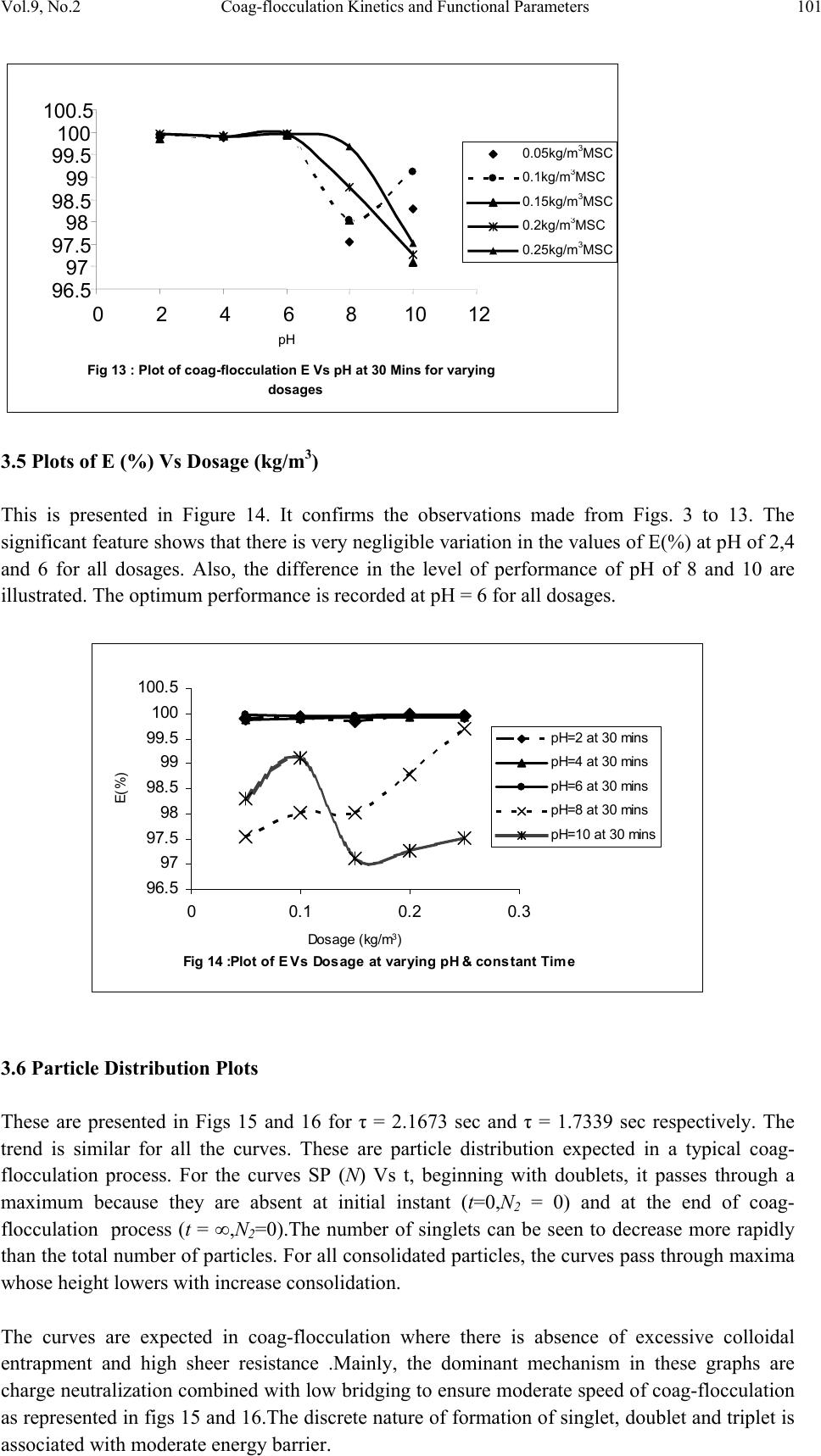

Vol.9, No.2 Coag-flocculation Kinetics and Functional Parameters 101
3.5 Plots of E (%) Vs Dosage (kg/m3)
This is presented in Figure 14. It confirms the observations made from Figs. 3 to 13. The
significant feature shows that there is very negligible variation in the values of E(%) at pH of 2,4
and 6 for all dosages. Also, the difference in the level of performance of pH of 8 and 10 are
illustrated. The optimum performance is recorded at pH = 6 for all dosages.
Fig 14 :Pl ot of E Vs Dosage at vary ing pH & c onstant Time
96.5
97
97.5
98
98.5
99
99.5
100
100.5
00.1 0.2 0.3
Dosage (kg/m
3
)
E(%)
pH=2 at 30 mins
pH=4 at 30 mins
pH=6 at 30 mins
pH=8 at 30 mins
pH=10 at 30 mins
3.6 Particle Distribution Plots
These are presented in Figs 15 and 16 for τ = 2.1673 sec and τ = 1.7339 sec respectively. The
trend is similar for all the curves. These are particle distribution expected in a typical coag-
flocculation process. For the curves SP (N) Vs t, beginning with doublets, it passes through a
maximum because they are absent at initial instant (t=0,N2 = 0) and at the end of coag-
flocculation process (t = ∞,N2=0).The number of singlets can be seen to decrease more rapidly
than the total number of particles. For all consolidated particles, the curves pass through maxima
whose height lowers with increase consolidation.
The curves are expected in coag-flocculation where there is absence of excessive colloidal
entrapment and high sheer resistance .Mainly, the dominant mechanism in these graphs are
charge neutralization combined with low bridging to ensure moderate speed of coag-flocculation
as represented in figs 15 and 16.The discrete nature of formation of singlet, doublet and triplet is
associated with moderate energy barrier.
Fig 13 : Plot of coag-flocculation E Vs pH at 30 Mins for varying
dosages
96.5
97
97.5
98
98.5
99
99.5
100
100.5
0 2 4 6 81012
pH
0.05kg/m
3
MSC
0.1kg/m
3
MSC
0.15kg/m
3
MSC
0.2kg/m
3
MSC
0.25kg/m
3
MSC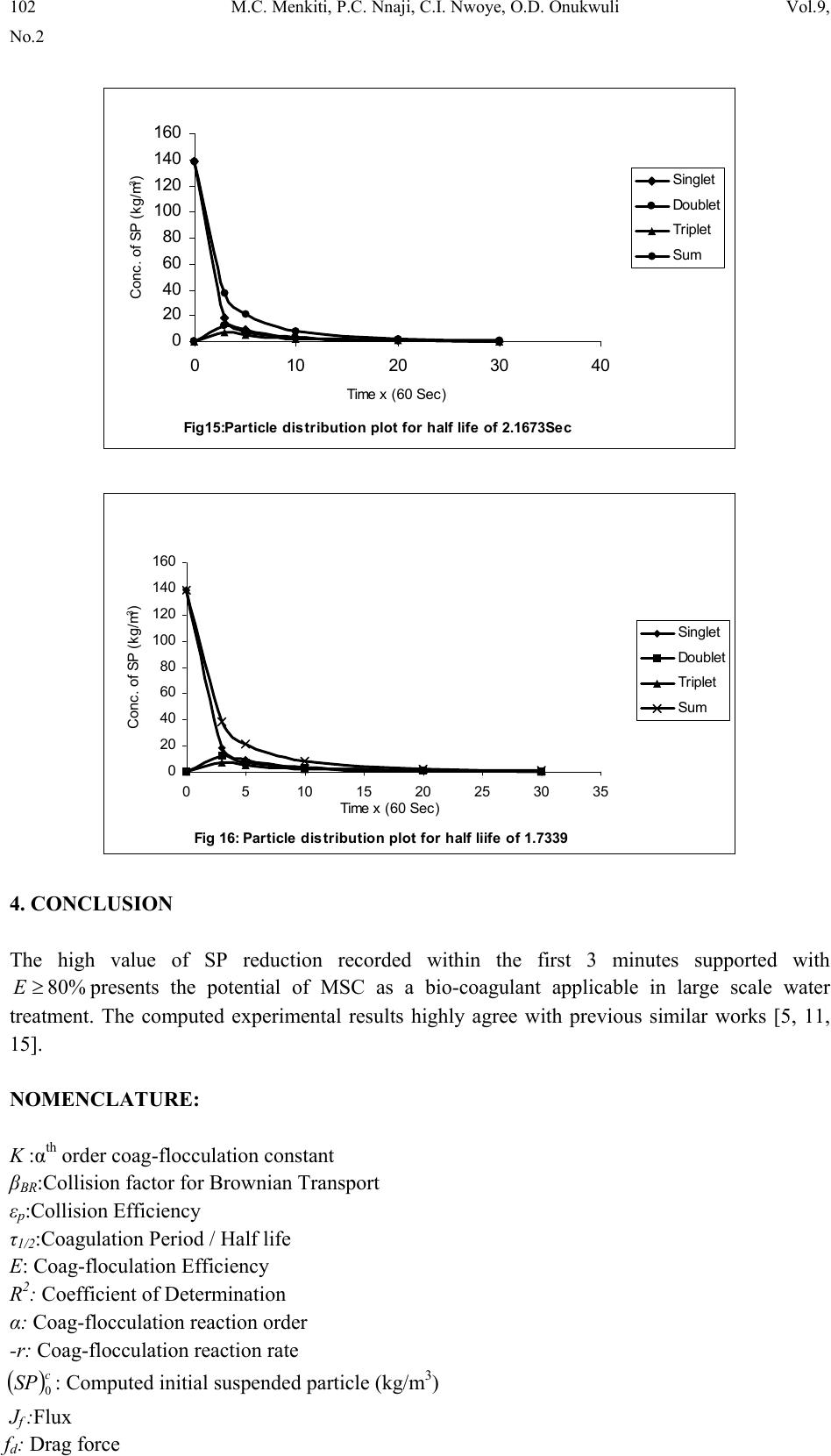

102 M.C. Menkiti, P.C. Nnaji, C.I. Nwoye, O.D. Onukwuli Vol.9,
No.2
Fig15:Particle distribution plot for half life of 2.1673Sec
0
20
40
60
80
100
120
140
160
0 10203040
Time x (60 Sec)
Conc. of SP (kg/m
3
)
Singlet
Doublet
Triplet
Sum
Fig 16: Particle distribution plot for half liife of 1.7339
0
20
40
60
80
100
120
140
160
0510 1520 2530 35
Time x (60 Sec)
Conc. of SP (kg/m
3
)
Singlet
Doublet
Triplet
Sum
4. CONCLUSION
The high value of SP reduction recorded within the first 3 minutes supported with
%80≥Epresents the potential of MSC as a bio-coagulant applicable in large scale water
treatment. The computed experimental results highly agree with previous similar works [5, 11,
15].
NOMENCLATURE:
K :αth order coag-flocculation constant
βBR:Collision factor for Brownian Transport
εp:Collision Efficiency
τ1/2:Coagulation Period / Half life
E: Coag-floculation Efficiency
R2: Coefficient of Determination
α: Coag-flocculation reaction order
-r: Coag-flocculation reaction rate
()
c
SP 0: Computed initial suspended particle (kg/m3)
Jf :Flux
fd: Drag force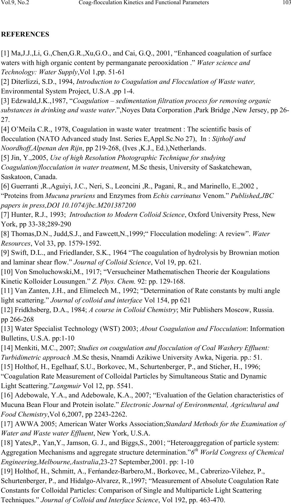

Vol.9, No.2 Coag-flocculation Kinetics and Functional Parameters 103
REFERENCES
[1] Ma,J.J.,Li, G.,Chen,G.R.,Xu,G.O., and Cai, G.Q., 2001, “Enhanced coagulation of surface
waters with high organic content by permanganate perooxidation .” Water science and
Technology: Water Supply,Vol 1,pp. 51-61
[2] Diterlizzi, S.D., 1994, Introduction to Coagulation and Flocculation of Waste water,
Environmental System Project, U.S.A ,pp 1-4.
[3] Edzwald,J.K.,1987, “Coagulation – sedimentation filtration process for removing organic
substances in drinking and waste water.”,Noyes Data Corporation ,Park Bridge ,New Jersey, pp 26-
27.
[4] O’Meila C.R., 1978, Coagulation in waste water treatment : The scientific basis of
flocculation (NATO Advanced study Inst. Series E,Appl.Sc.No 27), In : Sijtholf and
Noordhoff,Alpenan den Rijn, pp 219-268, (Ives ,K.J., Ed.),Netherlands.
[5] Jin, Y.,2005, Use of high Resolution Photographic Technique for studying
Coagulation/flocculation in water treatment, M.Sc thesis, University of Saskatchewan,
Saskatoon, Canada.
[6] Guerranti ,R.,Aguiyi, J.C., Neri, S., Leoncini ,R., Pagani, R., and Marinello, E.,2002 ,
“Proteins from Mucuna pruriens and Enzymes from Echis carrinatus Venom.” Published,JBC
papers in press,DOI 10.1074/jbc.M201387200
[7] Hunter, R.J., 1993; Introduction to Modern Colloid Science, Oxford University Press, New
York, pp 33-38;289-290
[8] Thomas,D.N., Judd,S.J., and Fawcett,N.,1999;“ Flocculation modeling: A review”. Water
Resources, Vol 33, pp. 1579-1592.
[9] Swift, D.L., and Friedlander, S.K., 1964 “The coagulation of hydrolysis by Brownian motion
and laminar shear flow.” Journal of Colloid Science, Vol 19, pp. 621.
[10] Von Smoluchowski,M., 1917; “Versucheiner Mathematischen Theorie der Koagulations
Kinetic Kolloider Lousungen.” Z. Phys. Chem. 92: pp. 129-168.
[11] Van Zanten, J.H., and Elimelech M., 1992; “Determination of Rate constants by multi angle
light scattering.” Journal of colloid and interface Vol 154, pp 621
[12] Fridkhsberg, D.A., 1984; A course in Colloid Chemistry; Mir Publishers Moscow, Russia.
pp 266-268
[13] Water Specialist Technology (WST) 2003; About Coagulation and Flocculation: Information
Bulletins, U.S.A. pp:1-10
[14] Menkiti, M.C., 2007; Studies on coagulation and flocculation of Coal Washery Effluent:
Turbidimetric approach .M.Sc thesis, Nnamdi Azikiwe University Awka, Nigeria. pp.: 51.
[15] Holthof, H., Egelhaaf, S.U., Borkovec, M., Schurtenberger, P., and Sticher, H., 1996;
“Coagulation Rate Measurement of Colloidal Particles by Simultaneous Static and Dynamic
Light Scattering.”Langmuir Vol 12, pp. 5541.
[16] Adebowale, Y.A., and Adebowale, K.A., 2007; “Evaluation of the Gelation characteristics of
Mucuna Bean Flour and Protein isolate.” Electronic Journal of Environmental, Agricultural and
Food Chemistry,Vol 6,2007, pp 2243-2262.
[17] AWWA 2005; American Water Works Association;Standard Methods for the Examination of
Water and Waste water Effluent, New York, U.S.A.
[18] Yates,P., Yan,Y., Jamson, G. J., and Biggs,S., 2001; “Heteroaggregation of particle system:
Aggregation Mechanisms and aggregate structure determination.”6th World Congress of Chemical
Engineering,Melbourne,Australia,23-27 September,2001. pp: 1-10
[19] Holthof, H., Schmitt, A., Ferńandez-Barbero,M., Borkovec, M., Cabrerizo-Vilehez, P.,
Schurtenberger, P., and Hidalgo-Alvarez, R.,1997; “Measurement of Absolute Coagulation Rate
Constants for Colloidal Particles: Comparison of Single and Multiparticle Light Scattering
Techniques.” Journal of Colloid and Interface Science, Vol 192, pp. 463-470.