 Open Journal of Statistics, 2012, 2, 251-259 http://dx.doi.org/10.4236/ojs.2012.23030 Published Online July 2012 (http://www.SciRP.org/journal/ojs) PC-VAR Estimation of Vector Autoregressive Models* Claudio Morana1,2,3,4 1Dipartimento di Economia Politica, Università di Milano Bicocca, Milano, Italy 2Center for Research on Pensions and Welfare Policies, Collegio Carlo Alberto, Moncalieri, Italy 3Fondazione Eni Enrico Mattei, Milano, Italy 4International Centre for Economic Research, ICER, Torino, Italy Email: claudio.morana@unimib.it Received May 7, 2012; revised June 8, 2012; accepted June 22, 2012 ABSTRACT In this paper PC-VAR estimation of vector autoregressive models (VAR) is proposed. The estimation strategy success- fully lessens the curse of dimensionality affecting VAR models, when estimated using sample sizes typically available in quarterly studies. The procedure involves a dynamic regression using a subset of principal components extracted from a vector time series, and the recovery of the implied unrestricted VAR parameter estimates by solving a set of lin- ear constraints. PC-VAR and OLS estimation of unrestricted VAR models show the same asymptotic properties. Monte Carlo results strongly support PC-VAR estimation, yielding gains, in terms of both lower bias and higher efficiency, relatively to OLS estimation of high dimensional unrestricted VAR models in small samples. Guidance for the selection of the number of components to be used in empirical studies is provided. Keywords: Vector Autoregressive Model; Principal Components Analysis; Statistical Reduction Techniques 1. Introduction In this paper principal components vector autoregressive estimation (PC-VAR) for large scale dynamic economet- ric models is proposed. Vector autoregressive models (VAR), when estimated using economic time series of sample sizes typically available in empirical quarterly studies, are subject to the curse of dimensionality. Recent contributions, dealing with this issue in the framework of factor augmented VAR (FVAR) models ([1-4]; see also [5] for a survey and new results), have mostly relied on principal components (PC) estimation (in the frequency or time domain) of the underlying unobserved common factor structure. Results of [1,6,7] have in fact proved consistency and asymptotic normality of PC estimation under various scenarios, including the exact and approxi- mate factor model case, weakly stationary (short memory) and I(1) integrated processes, also showing conditional heteroskedasticity; see also [8] for additional implica- tions of temporal dependence for PC estimation. The proposed approach is different from FVAR mod- eling, as no reference to an underlying factor structure is made, and PC estimation is performed to yield accurate estimation of the parameters of an unrestricted VAR model, rather than of a dynamic factor model. The pro- cedure involves a dynamic regression using a subset of principal components extracted from a vector time series, and the recovery of the implied unrestricted VAR pa- rameter estimates by solving a set of linear constraints. PC-VAR and OLS estimation of unrestricted VAR mod- els show the same asymptotic properties. Monte Carlo results strongly support PC-VAR estima- tion, yielding gains, in terms of both lower bias and higher efficiency, relatively to OLS estimation of high dimensional unrestricted VAR models in small samples. Guidance for the selection of the number of components to be used in empirical studies is provided. After this introduction, the paper is organized as fol- lows. In section two PC-VAR estimation is presented, while in section three Monte Carlo analysis is performed; see [9] for an empirical application of the procedure. 2. PC-VAR Estimation of VAR Models Consider the vector autoregressive (VAR) model .. ., tt tiid - 0, Σ IPL xη η t x1r (1) zero mean I(0) vector process, where is an 2 12 1, ,tT, and p LLL L PPP P has all the roots outside the unit circle, with P1, ,jp, ˆ ˆ tt Ξfx ˆˆ tt , being a square matrix of coefficients of order r. PC-VAR estimation relies on the following identity , (2) fΞx1r is the vector of estimated princi- where C opyright © 2012 SciRes. OJS  C. MORANA 252 pal components of t, is the matrix of or- thogonal eigenvectors associated with the r (ordered) eigenvalues of ( xˆ Ξ rr ˆ Σ tt Σ). This follows from the eigenvalue-eigenvector decomposition of, i.e., , where E xx Σ ˆˆ 1 ΞΣ ˆˆ Ξ=Γ ˆ , r1 ˆdi ˆ ,ag Γrr is the diagonal matrix containing the (ordered) eigenvalues of . ˆ Σ The validity of PC estimation for weakly dependent processes follows from results in [7] and [8]. In particu- lar, in [7], under some general conditions, r consis- tency and asymptotic normality of PC estimation of the unobserved common factors has been established, at each point in time, for and ,rT 0 L ˆˆ Ξx ˆ , t f 0Σ ε rT, when both the unobserved factors and the idiosyncratic components show limited serial correlation, and the latter also display limited heteroskedasticity in both their time-series and cross-sectional dimensions (see Theorem 1, p. 145); more- over, the invariance of the singular value decomposition to row ordering is discussed in [8] (see the Lemma on the eigenvalues matrix in [8], p. 175). PC-VAR estimation of is then be implemented as follows: P .. t tii xD ε 2 12 1) apply PCA to and compute f; ttt 2) obtain by means of OLS estimation of the stationary dynamic vector regression model x LD . L d t (3) where pLD ˆˆ L DΞ LLDD L D ˆ PCVAR LP has all the roots outside the unit circle; 3) recover the (implied OLS) estimate of the actual parameters yield by the unrestricted VAR model in (1) by solving the linear constraints . (4) Note that, by construction, the PC-VAR estimator and the OLS estimator of the unrestricted VAR model in (1) are the same estimator, i.e., ˆ PCVAR LLP ˆtt fη ˆˆˆ L ΞΞ P ΞΞ ˆ P OLS In fact, substituting (2) in (1) yields . t LxP ηε ˆ LLP ˆ Ξ, (5) i.e., the dynamic vector regression in (3), with and . ˆ LΞ LP D I LDP ˆ tt The implied matrix is then estimated by com- puting ˆˆ Ξ, as r due to the orthonormality of the eigenvec- tors. The PC-VAR estimator would therefore show the same asymptotic properties of the OLS estimator. ˆ The case considered is however of no interest for em- pirical implementations, as it does not allow for any di- mensionality reduction, relatively to the estimation of the unrestricted VAR model. 2.1. The Unfeasible Case Consider the case in which only the first s, r , prin- cipal components associated with the s largest ordered eigenvalues of are considered, with j ˆ Σˆ0 , j = s + 1, ···, r. The same results as obtained above ( r , im- plicitly) would hold. Rewrite the identity in (2) as ,,*,*, ˆˆ ˆˆ tsstrsrstt tt ΞfΞfxxτx *, , ˆ ˆ tsst Ξfx, ˆ ˆ trsrst (6) where , Ξf0τ, ˆrst as f0 ,, () (1)( ) () (1 )(1) ˆˆˆˆˆ ˆ '', tstrst srs rr rrsrrs srs , fff ΞΞΞ . Then, substituting (6) in (1) yields *,*, . tttttt LL xPx τηPxη (7) PC-VAR would then entail OLS estimation of , ˆ .. .,. tstt t L iid f 0Σ xD ε ε (8) It then follows ** ˆˆˆˆˆˆˆˆ 'LLL L DΞPΞPΞΞP, i.e., * ˆˆˆˆˆ PCVAR LLL PDΞDΞ, (9) 2 **1*2 * p LLL L DDD D *() () ,1,,, jj rrs rs LL jp 0DD , where 2 **1*2 * p LLL L PPP P *() () () () ˆˆ ,1,,, jjs j rrs rrs rs rr Ljp Ξ00ΞPP P and is the Hadamart product. 2.2. The Feasible Case rConsider the case in which only the first s, , prin- cipal components associated with the s largest ordered eigenvalues of are considered, with ˆ Σˆ0 j , j = s + 1, ···, r. By rewriting (7) as *, ,, , ˆˆ ˆˆ ˆ ˆ, tttt strsrstt sst t LL LL L x ΞfΞf Ξf PxPτη PP η Pλ where tt tt L ληPτη0 j , as, for , ˆrst , f0, Copyright © 2012 SciRes. OJS 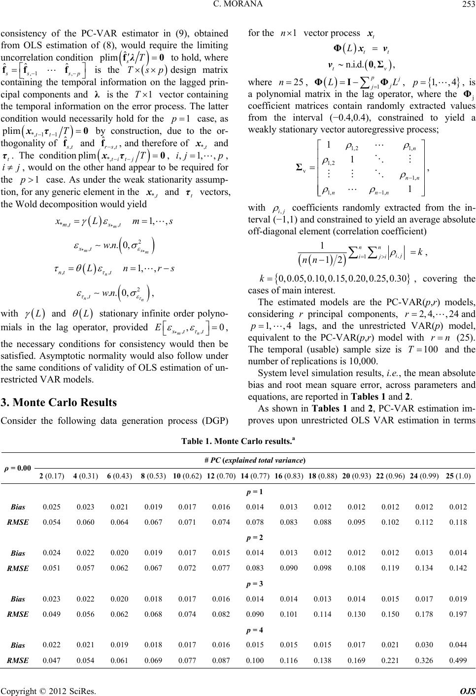 C. MORANA OJS 253 Copyright © 2012 SciRes. consistency of the PC-VAR estimator in (9), obtained from OLS estimation of (8), would require the limiting uncorrelation condition ˆ msT f0λpli ˆˆ to hold, where ,1 , ˆ ssp is the design matrix containing the temporal information on the lagged prin- cipal components and is the T vector containing the temporal information on the error process. The latter condition would necessarily hold for the case, as f λ ff Tsp 1 1p *, 11tt by construction, due to the or- thogonality of , plim xT0τ ˆ t and , and therefore of and . The condition f, ˆrs ft*,t x t τ *,titj, plim xT0 τ,1,,ij p t τ , , would on the other hand appear to be required for the case. As under the weak stationarity assump- tion, for any generic element in the and vectors, the Wold decomposition would yield ij p1 *,t x 1, , *m mt x*,, t Lms * 2 mx m , , *,.. xt wn ,, nt 0, 1Ln nt rs n E 2 0, ,.. ntwn L , with and stationary infinite order polyno- L mials in the lag operator, provided *,, ,0 mn xt t 1n , vector process t x for the n.i.d. ,, tt tv L Φ 0Σ xv v 25n the necessary conditions for consistency would then be satisfied. Asymptotic normality would also follow under the same conditions of validity of OLS estimation of un- restricted VAR models. 3. Monte Carlo Results Consider the following data generation process (DGP) where , 1 p j j, , is a polynomial matrix in the lag operator, where the j coefficient matrices contain randomly extracted values from the interval (−0.4,0.4), constrained to yield a weakly stationary vector autoregressive process; LL ΦIΦ 1,,4p Φ 1,2 1, 1,2 v 1, 1, 1, 1 1 1 n nn nnn Σ , with ,ij coefficients randomly extracted from the in- terval (−1,1) and constrained to yield an average absolute off-diagonal element (correlation coefficient) , 1 1 12 nn ij iji k nn , 0,0.05,0.10,0.15,0.20,0.25,0.30k 2, 4,, 24 1,,4p , covering the cases of main interest. The estimated models are the PC-VAR(p,r) models, considering r principal components, rand rn lags, and the unrestricted VAR(p) model, equivalent to the PC-VAR(p,r) model with (25). The temporal (usable) sample size is T and the number of replications is 10,000. 100 System level simulation results, i.e., the mean absolute bias and root mean square error, across parameters and equations, are reported in Tables 1 and 2. As shown in Tables 1 and 2, PC-VAR estimation im- proves upon unrestricted OLS VAR estimation in terms Table 1. Monte Carlo results.a # PC (explained total variance) ρ = 0.00 2 (0.17) 4 (0.31) 6 (0.43) 8 (0.53) 10 (0.62) 12 (0.70) 14 (0.77) 16 (0.83)18 (0.88) 20 (0.93) 22 (0.96) 24 (0.99) 25 (1.0) p = 1 Bias 0.025 0.023 0.021 0.019 0.017 0.016 0.014 0.013 0.012 0.012 0.012 0.012 0.012 RMSE 0.054 0.060 0.064 0.067 0.071 0.074 0.078 0.083 0.088 0.095 0.102 0.112 0.118 p = 2 Bias 0.024 0.022 0.020 0.019 0.017 0.015 0.014 0.013 0.012 0.012 0.012 0.013 0.014 RMSE 0.051 0.057 0.062 0.067 0.072 0.077 0.083 0.090 0.098 0.108 0.119 0.134 0.142 p = 3 Bias 0.023 0.022 0.020 0.018 0.017 0.016 0.014 0.014 0.013 0.014 0.015 0.017 0.019 RMSE 0.049 0.056 0.062 0.068 0.074 0.082 0.090 0.101 0.114 0.130 0.150 0.178 0.197 p = 4 Bias 0.022 0.021 0.019 0.018 0.017 0.016 0.015 0.015 0.015 0.017 0.021 0.030 0.044 RMSE 0.047 0.054 0.061 0.069 0.077 0.087 0.100 0.116 0.138 0.169 0.221 0.326 0.499 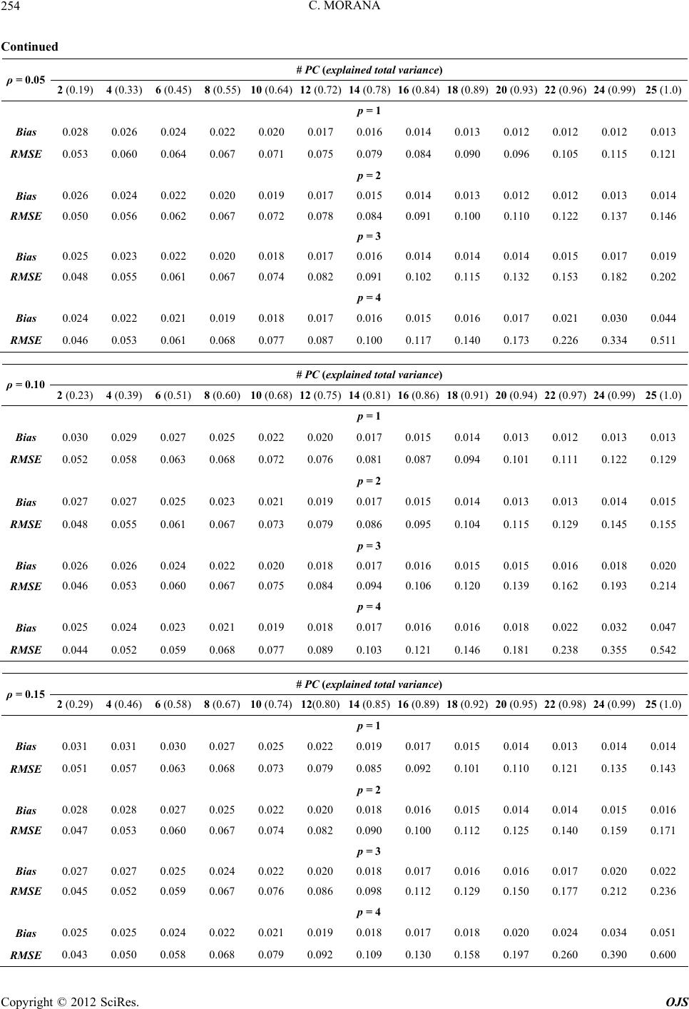 C. MORANA 254 Continued # PC (explained total variance) ρ = 0.05 2 (0.19) 4 (0.33) 6 (0.45) 8 (0.55) 10 (0.64)(0.89) 20 (0.93) 22 (0.96) 24 (0.99) 25 (1.0)12 (0.72) 14 (0.78) 16 (0.84) 18 p = 1 Bias 0.028 0.026 0.024 0.022 0.020 0.017 0.014 0.013 0.012 0.012 0.012 0.013 Bias 0.026 0.024 0.022 0.020 0.019 0.017 0.014 0.013 0.012 0.012 0.013 0.014 Bias 0.025 0.023 0.022 0.020 0.018 0.017 0.014 0.014 0.014 0.015 0.017 0.019 Bias 0.024 0.022 0.021 0.019 0.018 0.017 0.015 0.016 0.017 0.021 0.030 0.044 0.016 RMSE 0.053 0.060 0.064 0.067 0.071 0.075 0.079 0.084 0.090 0.096 0.105 0.115 0.121 p = 2 0.015 RMSE 0.050 0.056 0.062 0.067 0.072 0.078 0.084 0.091 0.100 0.110 0.122 0.137 0.146 p = 3 0.016 RMSE 0.048 0.055 0.061 0.067 0.074 0.082 0.091 0.102 0.115 0.132 0.153 0.182 0.202 p = 4 0.016 RMSE 0.046 0.053 0.061 0.068 0.077 0.087 0.100 0.117 0.140 0.173 0.226 0.334 0.511 # P) C (explained total variance ρ = 0.10 2 (0.23) 4 (0.39) 6 (0.51) 8 (0.60) 10 (0.68)(0.91) 20 (0.94) 22 (0.97) 24 (0.99) 25 (1.0)12 (0.75) 14 (0.81) 16 (0.86) 18 p = 1 Bias 0.030 0.029 0.027 0.025 0.022 0.020 0.015 0.014 0.013 0.012 0.013 0.013 Bias 0.027 0.027 0.025 0.023 0.021 0.019 0.015 0.014 0.013 0.013 0.014 0.015 Bias 0.026 0.026 0.024 0.022 0.020 0.018 0.016 0.015 0.015 0.016 0.018 0.020 Bias 0.025 0.024 0.023 0.021 0.019 0.018 0.016 0.016 0.018 0.022 0.032 0.047 0.017 RMSE 0.052 0.058 0.063 0.068 0.072 0.076 0.081 0.087 0.094 0.101 0.111 0.122 0.129 p = 2 0.017 RMSE 0.048 0.055 0.061 0.067 0.073 0.079 0.086 0.095 0.104 0.115 0.129 0.145 0.155 p = 3 0.017 RMSE 0.046 0.053 0.060 0.067 0.075 0.084 0.094 0.106 0.120 0.139 0.162 0.193 0.214 p = 4 0.017 RMSE 0.044 0.052 0.059 0.068 0.077 0.089 0.103 0.121 0.146 0.181 0.238 0.355 0.542 # P) C (explained total variance ρ = 0.15 2 (0.29) 4 (0.46) 6 (0.58) 8 (0.67) 10 (0.74)(0.92) 20 (0.95) 22 (0.98) 24 (0.99) 25 (1.0)12(0.80) 14 (0.85) 16 (0.89) 18 p = 1 Bias 0.031 0.031 0.030 0.027 0.025 0.022 0.017 0.015 0.014 0.013 0.014 0.014 Bias 0.028 0.028 0.027 0.025 0.022 0.020 0.016 0.015 0.014 0.014 0.015 0.016 Bias 0.027 0.027 0.025 0.024 0.022 0.020 0.017 0.016 0.016 0.017 0.020 0.022 Bias 0.025 0.025 0.024 0.022 0.021 0.019 0.017 0.018 0.020 0.024 0.034 0.051 0.019 RMSE 0.051 0.057 0.063 0.068 0.073 0.079 0.085 0.092 0.101 0.110 0.121 0.135 0.143 p = 2 0.018 RMSE 0.047 0.053 0.060 0.067 0.074 0.082 0.090 0.100 0.112 0.125 0.140 0.159 0.171 p = 3 0.018 RMSE 0.045 0.052 0.059 0.067 0.076 0.086 0.098 0.112 0.129 0.150 0.177 0.212 0.236 p = 4 0.018 RMSE 0.043 0.050 0.058 0.068 0.079 0.092 0.109 0.130 0.158 0.197 0.260 0.390 0.600 Copyright © 2012 SciRes. OJS 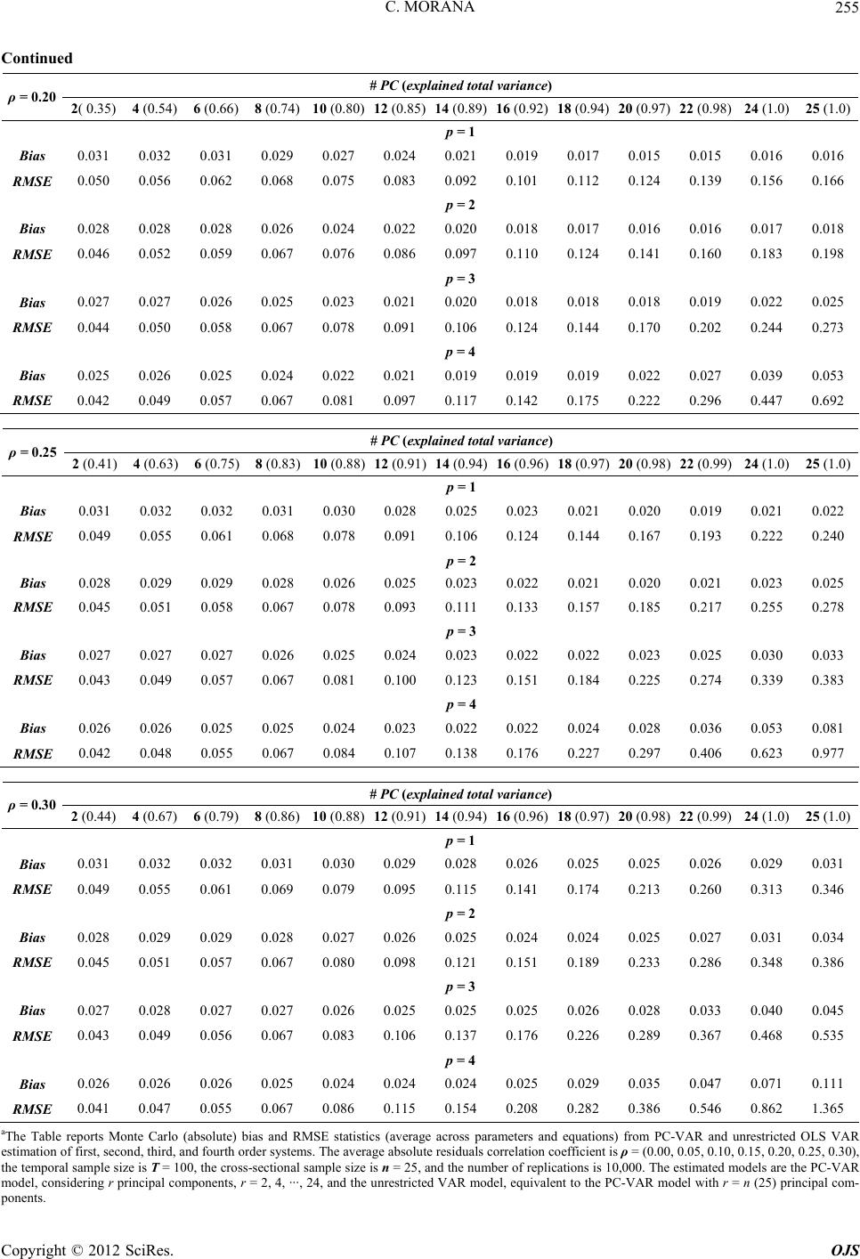 C. MORANA 255 Continued # PC (explained total variance) ρ = 0.20 2( 0.35) 4 (0.54) 6 (0.66) 8 (0.74) 10 (0.80)(0.94) 20 (0.97) 22 (0.98) 24 (1.0) 25 (1.0)12 (0.85) 14 (0.89) 16 (0.92) 18 p = 1 Bias 0.031 0.032 0.031 0.029 0.027 0.024 0.019 0.017 0.015 0.015 0.016 0.016 Bias 0.028 0.028 0.028 0.026 0.024 0.022 0.018 0.017 0.016 0.016 0.017 0.018 Bias 0.027 0.027 0.026 0.025 0.023 0.021 0.018 0.018 0.018 0.019 0.022 0.025 Bias 0.025 0.026 0.025 0.024 0.022 0.021 0.019 0.019 0.022 0.027 0.039 0.053 0.021 RMSE 0.050 0.056 0.062 0.068 0.075 0.083 0.092 0.101 0.112 0.124 0.139 0.156 0.166 p = 2 0.020 RMSE 0.046 0.052 0.059 0.067 0.076 0.086 0.097 0.110 0.124 0.141 0.160 0.183 0.198 p = 3 0.020 RMSE 0.044 0.050 0.058 0.067 0.078 0.091 0.106 0.124 0.144 0.170 0.202 0.244 0.273 p = 4 0.019 RMSE 0.042 0.049 0.057 0.067 0.081 0.097 0.117 0.142 0.175 0.222 0.296 0.447 0.692 # P) C (explained total variance ρ = 0.25 2 (0.41) 4 (0.63) 6 (0.75) 8 (0.83) 10 (0.88)(0.97)20 (0.98) 22 (0.99) 24 (1.0) 25 (1.0)12 (0.91) 14 (0.94) 16 (0.96) 18 p = 1 Bias 0.031 0.032 0.032 0.031 0.030 0.028 0.023 0.021 0.020 0.019 0.021 0.022 RMSE Bias 0.028 0.029 0.029 0.028 0.026 0.025 0.022 0.021 0.020 0.021 0.023 0.025 RMSE Bias 0.027 0.027 0.027 0.026 0.025 0.024 0.022 0.022 0.023 0.025 0.030 0.033 RMSE Bias 0.026 0.026 0.025 0.025 0.024 0.023 0.022 0.024 0.028 0.036 0.053 0.081 RMSE 0.025 0.049 0.055 0.061 0.068 0.078 0.091 0.106 0.124 0.144 0.167 0.193 0.222 0.240 p = 2 0.023 0.045 0.051 0.058 0.067 0.078 0.093 0.111 0.133 0.157 0.185 0.217 0.255 0.278 p = 3 0.023 0.043 0.049 0.057 0.067 0.081 0.100 0.123 0.151 0.184 0.225 0.274 0.339 0.383 p = 4 0.022 0.042 0.048 0.055 0.067 0.084 0.107 0.138 0.176 0.227 0.297 0.406 0.623 0.977 # P) C (explained total variance ρ = 0.30 2 (0.44) 4 (0.67) 6 (0.79) 8 (0.86) 10 (0.88)(0.97) 20 (0.98) 22 (0.99) 24 (1.0) 25 (1.0)12 (0.91) 14 (0.94) 16 (0.96) 18 p = 1 Bias 0.031 0.032 0.032 0.031 0.030 0.029 0.026 0.025 0.025 0.026 0.029 0.031 Bias 0.028 0.029 0.029 0.028 0.027 0.026 0.024 0.024 0.025 0.027 0.031 0.034 Bias 0.027 0.028 0.027 0.027 0.026 0.025 0.025 0.026 0.028 0.033 0.040 0.045 Bias 0.026 0.026 0.026 0.025 0.024 0.024 0.025 0.029 0.035 0.047 0.071 0.111 0.028 RMSE 0.049 0.055 0.061 0.069 0.079 0.095 0.115 0.141 0.174 0.213 0.260 0.313 0.346 p = 2 0.025 RMSE 0.045 0.051 0.057 0.067 0.080 0.098 0.121 0.151 0.189 0.233 0.286 0.348 0.386 p = 3 0.025 RMSE 0.043 0.049 0.056 0.067 0.083 0.106 0.137 0.176 0.226 0.289 0.367 0.468 0.535 p = 4 0.024 RMSE 0.041 0.047 0.055 0.067 0.086 0.115 0.154 0.208 0.282 0.386 0.546 0.862 1.365 aT reon (abMSticse arams) -Vund OLS VAR scond, and foms. Trage ae reorreoet is ρ 0. 0.15, 0.2), he Table timation of firs ports M t, se te Carlo third, solute) bia urth orde s and R r syste E statis he ave (averag bsolut cross pa siduals c eters and e lation c quation fficien from PC = (0.00, AR and 05, 0.10, restricte 0.20,e the temporal sample size is T = 100, the cross-sectional sample size is n = 25, and the number of replications is 10,000. The estimated models are the PC-VAR model, considering r principal components, r = 2, 4, ···, 24, and the unrestricted VAR model, equivalent to the PC-VAR model with r = n (25) principal com- ponents. 5, 0.30 Copyright © 2012 SciRes. OJS 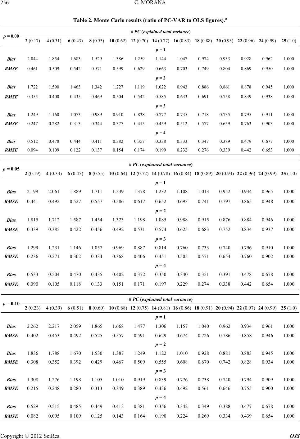 C. MORANA 256 Table 2. Monte Carlo results (ratio of PC-VAR to OLS figures).a # PC (explained total variance) ρ = 0.00 2 (0.17) 4 (0.31) 6 (0.43) 8 (0.53) 10 (0.62) 18 (0.88) 20 (0.93) 22 (0.96) 24 (0.99) 25 (1.0)12 (0.70) 14 (0.77) 16 (0.83) p = 1 Bis 2.044 1.854 1.683 1.529 1.386 1.259 1.047 0.974 0.933 0.928 0.962 1.000 R Bis 1.722 1.590 1.463 1.342 1.227 1.119 0.943 0.886 0.861 0.878 0.945 1.000 R Bis 1.249 1.160 1.073 0.989 0.910 0.838 0.735 0.718 0.735 0.795 0.911 1.000 R Bis 0.512 0.478 0.444 0.411 0.382 0.357 0.333 0.347 0.389 0.479 0.677 1.000 R a1.144 MSE 0.461 0.509 0.542 0.571 0.599 0.629 0.663 0.703 0.749 0.804 0.869 0.950 1.000 p = 2 a1.022 MSE 0.355 0.400 0.435 0.469 0.504 0.542 0.585 0.633 0.691 0.758 0.839 0.938 1.000 p = 3 a0.777 MSE 0.247 0.282 0.313 0.344 0.377 0.415 0.459 0.512 0.577 0.659 0.763 0.903 1.000 p = 4 a0.338 MSE 0.094 0.109 0.122 0.137 0.154 0.174 0.199 0.232 0.276 0.339 0.442 0.653 1.000 # P) C (explained total variance ρ = 0.05 2 (0.19) 4 (0.33) 6 (0.45) 8 (0.55) 10 (0.64)(0.89) 20 (0.93) 22 (0.96) 24 (0.99) 25 (1.0)12 (0.72) 14 (0.78) 16 (0.84) 18 p = 1 Bias 2.199 2.061 1.889 1.711 1.539 1.378 1.108 1.013 0.952 0.934 0.965 1.000 Bias 1.815 1.712 1.587 1.454 1.323 1.198 0.988 0.915 0.876 0.884 0.946 1.000 Bias 1.299 1.231 1.146 1.057 0.969 0.887 0.760 0.733 0.740 0.796 0.910 1.000 Bias 0.533 0.504 0.470 0.435 0.402 0.372 0.340 0.351 0.391 0.478 0.678 1.000 1.232 RMSE 0.441 0.492 0.527 0.557 0.586 0.617 0.652 0.693 0.741 0.797 0.865 0.948 1.000 p = 2 1.085 RMSE 0.339 0.385 0.422 0.456 0.492 0.531 0.574 0.625 0.683 0.752 0.834 0.937 1.000 p = 3 0.814 RMSE 0.236 0.271 0.302 0.334 0.368 0.406 0.451 0.505 0.571 0.654 0.760 0.902 1.000 p = 4 0.350 RMSE 0.090 0.105 0.118 0.133 0.151 0.171 0.197 0.229 0.274 0.338 0.442 0.654 1.000 # P) C (explained total variance ρ = 0.10 2 (0.23) 4 (0.39) 6 (0.51) 8 (0.60) 10 (0.68)(0.91) 20 (0.94) 22 (0.97) 24 (0.99) 25 (1.0)12 (0.75) 14 (0.81) 16 (0.86) 18 p = 1 Bias 2.262 2.217 2.059 1.865 1.668 1.477 1.157 1.040 0.962 0.934 0.961 1.000 Bias 1.836 1.788 1.670 1.530 1.387 1.249 1.010 0.928 0.881 0.883 0.945 1.000 Bias 1.308 1.276 1.198 1.105 1.010 0.919 0.776 0.738 0.740 0.794 0.909 1.000 Bias 0.529 0.515 0.485 0.449 0.413 0.381 0.342 0.349 0.388 0.477 0.678 1.000 RMSE 0.082 0.095 0.109 0.125 0.143 0.164 0.190 0.224 0.269 0.334 0.439 0.654 1.000 1.306 RMSE 0.402 0.453 0.492 0.525 0.557 0.591 0.629 0.674 0.726 0.786 0.858 0.946 1.000 p = 2 1.122 RMSE 0.308 0.352 0.392 0.429 0.467 0.509 0.555 0.608 0.670 0.742 0.828 0.934 1.000 p = 3 0.839 RMSE 0.215 0.248 0.280 0.313 0.349 0.389 0.436 0.492 0.561 0.646 0.755 0.900 1.000 p = 4 0.356 Copyright © 2012 SciRes. OJS 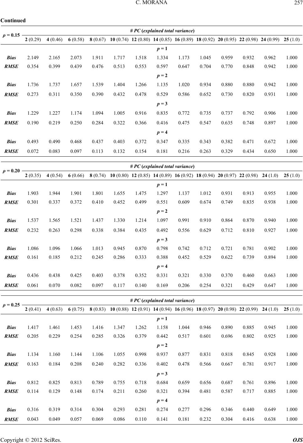 C. MORANA 257 Continued # lal v) PC (expined totaariance ρ = 0.15 2 (0.29) 4 (0.46) 6 (0.58) 8 (0.67) 10 (0.74) 12 (0.80) 14 (0.85) 16 (0.89)18 (0.92) 20 (0.95) 22 (0.98) 24 (0.99) 25 (1.0) p = 1 Bias 2.149 2.165 2.073 1.911 1.717 1.518 1.334 1.173 1.045 0.959 0.932 0.962 1.000 RMSE 0.354 0.399 0.439 0.476 0.513 0.553 0.647 0.704 0.770 0.848 0.942 1.000 RMSE 0.273 0.311 0.350 0.390 0.432 0.478 0.586 0.652 0.730 0.820 0.931 1.000 RMSE 0.190 0.219 0.250 0.284 0.322 0.366 0.475 0.547 0.635 0.748 0.897 1.000 RMSE 0.072 0.083 0.097 0.113 0.132 0.154 0.216 0.263 0.329 0.434 0.650 1.000 0.597 p = 2 Bias 1.736 1.737 1.657 1.539 1.404 1.266 1.135 1.020 0.934 0.880 0.880 0.942 1.000 0.529 p = 3 Bias 1.229 1.227 1.174 1.094 1.005 0.916 0.835 0.772 0.735 0.737 0.792 0.906 1.000 0.416 p = 4 Bias 0.493 0.490 0.468 0.437 0.403 0.372 0.347 0.335 0.343 0.382 0.471 0.672 1.000 0.181 # P) C (explained total variance ρ = 0.20 2 4 6 8 10 12 14 16 18 20 22 24 25 (0.35) (0.54) (0.66) (0.74)(0.80) (0.85) (0.89) (0.92)(0.94) (0.97) (0.98)(1.0) (1.0) p = 1 Bias 1.903 1.944 1.901 1.801 1.655 1.475 1.297 1.137 1.012 0.931 0.913 0.955 1.000 RMSE 0.301 0.337 0.372 0.410 0.452 0.499 0.609 0.674 0.749 0.835 0.938 1.000 RMSE 0.232 0.263 0.298 0.338 0.384 0.435 0.556 0.629 0.712 0.810 0.927 1.000 RMSE 0.161 0.185 0.212 0.245 0.286 0.333 0.452 0.529 0.622 0.739 0.894 1.000 RMSE 0.061 0.070 0.082 0.097 0.117 0.140 0.206 0.254 0.321 0.429 0.647 1.000 0.551 p = 2 Bias 1.537 1.565 1.521 1.437 1.330 1.214 1.097 0.991 0.910 0.864 0.870 0.940 1.000 0.492 p = 3 Bias 1.086 1.096 1.066 1.013 0.945 0.870 0.798 0.742 0.712 0.721 0.781 0.902 1.000 0.388 p = 4 Bias 0.436 0.438 0.425 0.403 0.378 0.352 0.331 0.321 0.330 0.370 0.460 0.663 1.000 0.169 # P) C (explained total variance ρ = 0.25 2 4 6 8 10 12 14 16 18 20 22 24 25 (0.41) (0.63) (0.75) (0.83)(0.88) (0.91) (0.94) (0.96)(0.97) (0.98) (0.99)(1.0) (1.0) p = 1 Bias 1.417 1.461 1.453 1.416 1.347 1.262 1.158 1.044 0.946 0.890 0.885 0.945 1.000 RMSE 0.205 0.229 0.254 0.285 0.326 0.379 0.517 0.601 0.696 0.802 0.925 1.000 RMSE 0.163 0.184 0.208 0.240 0.282 0.336 0.478 0.566 0.667 0.781 0.917 1.000 RMSE 0.114 0.129 0.148 0.174 0.211 0.260 0.394 0.481 0.587 0.717 0.885 1.000 RMSE 0.043 0.049 0.057 0.069 0.086 0.110 0.181 0.232 0.304 0.416 0.638 1.000 0.442 p = 2 Bias 1.134 1.160 1.144 1.106 1.055 0.998 0.937 0.877 0.831 0.818 0.845 0.928 1.000 0.402 p = 3 Bias 0.812 0.825 0.813 0.789 0.755 0.718 0.684 0.659 0.656 0.687 0.761 0.896 1.000 0.321 p = 4 Bias 0.316 0.319 0.314 0.304 0.293 0.281 0.274 0.277 0.296 0.346 0.440 0.649 1.000 0.141 Copyright © 2012 SciRes. OJS 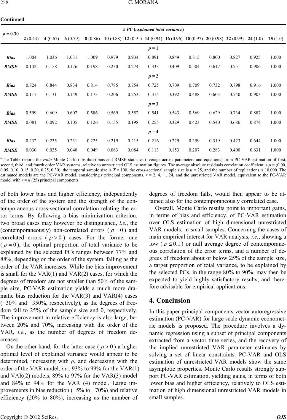 C. MORANA Copyright © 2012 SciRes. OJS 258 Continued # lal v) PC (expined totaariance ρ = 0.30 2 (0.44) 4 (0.67) 6 (0.79) 8 (0.86) 10 (0.88) 12 (0.91) 14 (0.94) 16 (0.96)18 (0.97) 20 (0.98) 22 (0.99) 24 (1.0) 25 (1.0) p = 1 Bias 1.004 1.036 1.031 1.009 0.979 0.934 0.891 0.849 0.815 0.800 0.827 0.925 1.000 RMSE 0.142 0.158 0.176 0.198 0.230 0.274 0.409 0.504 0.617 0.751 0.906 1.000 RMSE 0.117 0.131 0.149 0.173 0.206 0.253 0.392 0.488 0.603 0.740 0.903 1.000 RMSE 0.081 0.092 0.105 0.126 0.155 0.198 0.329 0.423 0.540 0.686 0.874 1.000 RMSE 0.030 0.035 0.040 0.049 0.063 0.084 0.153 0.207 0.283 0.400 0.631 1.000 0.333 p = 2 Bias 0.824 0.844 0.834 0.814 0.785 0.754 0.725 0.709 0.709 0.732 0.798 0.916 1.000 0.314 p = 3 Bias 0.599 0.609 0.602 0.586 0.569 0.552 0.541 0.543 0.569 0.629 0.734 0.887 1.000 0.255 p = 4 Bias 0.232 0.235 0.231 0.225 0.219 0.215 0.216 0.229 0.259 0.319 0.423 0.644 1.000 0.113 aThe ree rntebsias SEs (acrme eq froARtiot, sed, ath orAR systes, red Oation figres. Teragete reorr coeft is ρ 0. 0. thraless-l sae i anmb 10,e e strength of the con- e Tablports thatio Mo Carlo (aolute) band RM statisticverage aoss paraters anduations)m PC-V estiman of firs cond, thir 05, 0.10, 0. nd four 15, 0.20, der V 25, 0.30), m e tempo lative to unre sample siz stricte is T = 100, LS estim the cro u sectiona he av mple siz absolu s n = 25, siduals c d the nu elation er of replic ficien ations is = (0.00, 000. Th estimated models are the PC-VAR model, considering r principal components, r = 2, 4, ···, 24, and the unrestricted VAR model, equivalent to the PC-VAR model with r = n (25) principal components. of both lower bias and higher efficiency, independently of the order of the system and th temporaneous cross-sectional correlation relating the er- ror terms. By following a bias minimization criterion, two broad cases may however be distinguished, i.e., the (contemporaneously) non-correlated errors (0 ) and correlated errors (0 ) cases. For the former one (0 ), the optimal proportion of total variance to be explained by the selected PCs ranges between 77% and 88%, depending on the order of the system, falling as the order of the VAR increases. While the bias improvement is small for the VAR(1) and VAR(2) cases, for which the degrees of freedom are not smaller than 50% of the sam- ple size, PC-VAR estimation yields a much more dra- matic bias reduction for the VAR(3) and VAR(4) cases (−30% and −350%, respectively), as the degrees of free- dom fall to 25% of the sample size and 0, respectively. The improvement in relative efficiency is also large, be- tween 20% and 70%, increasing with the order of the VAR, i.e., as the number of degrees of freedom de- creases. On the other hand, for the latter case (0 ) a higher optimal level of explained variance would appear to be determined, increasing with ρ, and decrth the order of the VAR model, i.e., 93% to 99% for the VAR(1) and VAR(2) models, 89% to 97% for the VAR(3) model and 84% to 94% for the VAR (4) model. Large im- provements in bias reduction (−5% to −70%) and relative efficiency (20% to 80%), increasing as the number of Overall, Monte Carlo results point to important gains, in terms of bias and efficiency, of PC-VAR estimation over OLS estimation of high dimensional unrestricted VAR models, in small samples. Concerning the cases of main empirical interest for VAR analysis, i.e., showing a low (0.1 easing wi tained also for the contemporaneously correlated case. degrees of freedom falls, would then appear to be at- ) or null average degree of contemporane- ous correlation of the error terms, and a number of de- grees of freedom about or below 25% of the sample size, a target proportion of total variance, to be explained by the selected PCs, in the range 80% to 90%, may then be expected to yield highly satisfactory results, and there- fore advisable for empirical applications. 4. Conclusion In this paper principal components vector autoregressive estimation (PC-VAR) for large scale dynamic economet- ric models is proposed. The procedure involves a dy- namic regression using a subset of principal components ector time series, and the recovery of extracted from a v the implied unrestricted VAR parameter estimates by solving a set of linear constraints. PC-VAR and OLS estimation of unrestricted VAR models show the same asymptotic properties. Monte Carlo results strongly sup- port PC-VAR estimation, yielding gains, in terms of both lower bias and higher efficiency, relatively to OLS esti- mation of high dimensional unrestricted VAR models in small samples.  C. MORANA 259 5. Acknowledgements The author is grateful to two anonymous referees of the OJS for constructive comments. REFERENCES nic Attack on Unit Roots and ica, Vol. 72, No. 4, 2004, pp. [1] J. Bai and S. Ng, “A Pa Cointegration,” Econometr 1127-1177. doi:10.1111/j.1468-0262.2004.00528 [2] B. S. Bernanke and J. Boivin, “Monetary Policy in a Data- Rich Environment,” Journal of Monetary Economics, Vo 50, No. 3, 2003, pp. 525-546. doi:10.1016/S l. 0304-3932(03)00024-2 [3] M. Forni, M. Hallin, M. Lippi and L. Reichlin, “The Gen- eralized Dynamic Factor Model: Identification and Esti- mation,” Review of Economics and Statistics, Vol. 82, No. 4, 2000, pp. 540-554. doi:10.1162/003465300559037 ” Journal of Busi- [4] M. H. Pesaran, T. Schuerman and S. M. Weiner, “Model- ling Regional Interdependencies Using a Global Error Correcting Macroeconometric Model, ness and Economic Statistics, Vol. 22, No. 2, 2004, pp. 129-162. doi:10.1198/073500104000000019 [5] C. Morana, “Factor Vector Autoregressive Estimation of Heteroskedastic Persistent and Non Persistent Processes Subject to Structural Breaks,” 2011. http://ssrn.com/abstract=1756376 [6] J. Bai, “Estimating Cross-Section Common Stochastic Trends in Nonstationary Panel Data,” metrics, Vol. 122, No. 1, 2004, pp. 137-38 Journal of Econo- . doi:10.1016/j.jeconom.2003.10.022 [7] J. Bai, “Inferential Theory for Factor Models of Large Dimensions”, Econometrica, Vol. 71, No. 1, 20 171. 03, pp. 135- doi:10.1111/1468-0262.00392 [8] J. R. G. Lansang and E. B. Barrios, “Principal Compo- nents Analyisis of Nonstationary Time Series Data,” Sta- tistics and Computing, Vol. 19, No. 2, 2009, pp. 173-187. doi:10.1007/s11222-008-9082-y [9] C. Morana, “Oil Price Dynamics, Macro-Finance Interac- tions and the Role of Financial Speculation,” FEEM Working Paper Series, No. 7, 2011. http://ssrn.com/abstract=2025787 Copyright © 2012 SciRes. OJS
|