Open Journal of Statistics, 2012, 2, 313-318
http://dx.doi.org/10.4236/ojs.2012.23039 Published Online July 2012 (http://www.SciRP.org/journal/ojs)
An Exceptional Generalization of the Poisson Distribution
Per-Erik Hagmark
Department of Mechanics and Design, Tampere University of Technology, Tampere, Finland
Received May 4, 2012; revised June 10, 2012; accepted June 23, 2012
ABSTRACT
A new two-parameter count distribution is derived starting with probabilistic arguments around the gamma function and
the digamma function. This model is a generalization of the Poisson model with a noteworthy assortment of qualities.
For example, the mean is the main model parameter; any possible non-trivial variance or zero probability can be at-
tained by changing the other model parameter; and all distributions are visually natural-shaped. Thus, exact modeling to
any degree of over/under-dispersion or zero-inflation/deflation is possible.
Keywords: Count Data; Gamma Function; Poisson Generalization; Discretization; Modeling; Over/Under-Dispersion;
Zero-Inflation/Deflation
1. Introduction and the Main Result
In count data modeling the Poisson distribution is usually
the first option, but real data can indicate a variety of
discrepancies. These can be genuine features or secon-
dary consequences of e.g. censoring, clustering, approxi-
mations or correlations. Specifically, the Poisson model
has no dispersion flexibility because the mean determines
the variance and the zero probability, σ2 = μ, p0 = e–μ,
while the real data can display over or under- dispersion,
σ2 ≠ μ, or zero-inflation or deflation, p0 ≠ e–μ [1]. Such
situations are usually handled e.g. by randomizing the
Poisson mean, by mixtures, by adding a new parameter,
by reweighing the Poisson point probabilities, or via
generalizing the exponential increments in the homoge-
neous Poisson process [2-5]. Our approach will be dif-
ferent.
We recall an elementary fact. The mean-deviation pair
(μ, σ) of a non-binary count variable (non-negative inte-
ger-valued random variable) always satisfies the inequal-
ity


 


1
2

   , (1)
where [μ] is the largest integer not exceeding μ. Thus, we
will say that a count model (parameterized count variable)
has full dispersion flexibility if every positive solution (μ,
σ) of the inequality (1) is the mean-deviation pair for
some parameter values.
In [6] we called for a mathematically unified count
model N(μ, β) with two independent parameters, µ > 0, β
> 0, and the following properties:
1) Comfortable parameterization: E(N(μ, β)) = μ, for
all μ and β.
2) Generalization of the Poisson model: For β = 1,




Pr ,1!
n
Nμne n



, n = 0, 1, ···.
3) Full dispersion flexibility: If the numbers μ > 0 and
σ > 0 satisfy inequality (1), then there is a β such that


 
2
Var ,N  .

The solution to be presented in this paper obeys the
following cumulative probabilities:


 

 
Pr
1,,1
11
1, 1,1,
Nμ,βn
nn
nG ng
nn
nG ng

 

 

 
 
 
 
 

 
 
 
(2)
where g(t, x) and G(t, x) are the one-parameter gamma
probability and cumulative distribution functions, respec-
tively, with parameter x and variable t (Section 2).
We begin with the derivation of fundamental inequali-
ties in Section 2. These inequalities lead to a cumulative
distribution H(x, μ), where the parameter μ > 0 is the
mean. Then the insertion of a new independent parameter
β > 0 provides an extended cumulative distribution H(x/β,
μ/β) and the related non-negative two-parameter random
variable X(μ, β), where μ is still the mean. Now the pro-
claimed count model N(μ, β) is defined as a mean-pre-
serving discretization of X(μ, β), and the above properties
1), 2), 3) are proved. Thereafter the most immediate ap-
plications are given; namely, exact modeling of over/
under-dispersion or zero-inflation/deflation to any possi-
ble degree. In the last section, we propose motives for
further research, and we compare N(μ, β) with well-es-
tablished Poisson generalizations.
C
opyright © 2012 SciRes. OJS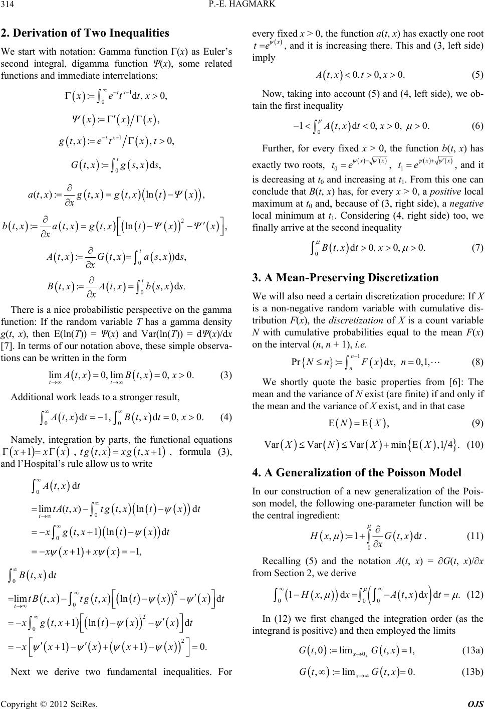

P.-E. HAGMARK 314
2. Derivation of Two Inequalities
We start with notation: Gamma function Г(x) as Euler’s
second integral, digamma function Ψ(x), some related
functions and immediate interrelations;

0
xe


1
:d,0,
tx
ttx
 
  
:,
x
xx





1
,: tx gtxe t
 , 0,x t

0,d,
tgsxs


,:Gtx 
 
(, ):,,lat xgt xgt x
x
  
n ,t x   



   
2
,:,, ln,btxatx gtxtxx 


 



x


 
0
,: ,,)d,
t
A
txGtxasx s
x




 
,: ,Btx Atx

0,d.
tbsxs
x



 
lim ,0,lim ,0,0
tt
AtxBtx x
 


00
,d1,,d 0,0Atx tBtx tx 

There is a nice probabilistic perspective on the gamma
function: If the random variable T has a gamma density
g(t, x), then E(ln(T)) = Ψ(x) and Var(ln(T)) = dΨ(x)/dx
[7]. In terms of our notation above, these simple observa-
tions can be written in the form
. (3)
Additional work leads to a stronger result,


 . (4)
Namely, integration by parts, the functional equations
 
1
x
xx
 
,tgtx xgtx,, formula (3),
and l’Hospital’s rule allow us to write

,1
  
 
0
d
d
,
tx t
x t
 


 
2
2
d
d
0.
x t
xt
x
















,dAtx t




 
0
0
lim(,),ln
,1ln
11
tt
Atx tgtx
xgtx t
xx xx






 
 



0,dBtx t


  

 

 
0
2
0
lim ,, ln
,1ln
11
tt
Btx tgtxtx
xgtxtx
xxx x

 



 






 


Next we derive two fundamental inequalities. For
every fixed x > 0, the function a(t, x) has exactly one root
x
te

, and it is increasing there. This and (3, left side)
imply


,0,0,0.Atxtx



0
1,d0,0, 0.Atx tx


(5)
Now, taking into account (5) and (4, left side), we ob-
tain the first inequality


 
(6)

Further, for every fixed x > 0, the function b(t, x) has
exactly two roots, 0
x
x
te




 
, 1
x
x
te





0,d 0,0,0Btx tx
, and it
is decreasing at t0 and increasing at t1. From this one can
conclude that B(t, x) has, for every x > 0, a positive local
maximum at t0 and, because of (3, right side), a negative
local minimum at t1. Considering (4, right side) too, we
finally arrive at the second inequality

.  

 
1
Pr:d,0,1,
n
n
Nn Fxxn

 

(7)
3. A Mean-Preserving Discretization
We will also need a certain discretization procedure: If X
is a non-negative random variable with cumulative dis-
tribution F(x), the discretization of X is a count variable
N with cumulative probabilities equal to the mean F(x)
on the interval (n, n + 1), i.e.
(8)
We shortly quote the basic properties from [6]: The
mean and the variance of N exist (are finite) if and only if
the mean and the variance of X exist, and in that case


EE,NX (9)



  
VarVarVarminE,14.XNXX

(10)
4. A Generalization of the Poisson Model
In our construction of a new generalization of the Pois-
son model, the following one-parameter function will be
the central ingredient:

0
,:1 ,d
H
xGtxt
x









000
1,d,ddHxxAtx x t

. (11)
Recalling (5) and the notation A(t, x) = ∂G(t, x)/∂x
from Section 2, we derive
.




 
 (12)
In (12) we first changed the integration order (as the
integrand is positive) and then employed the limits


0
,0 :lim,1,
x
Gt Gtx

 (13a)




,:lim, 0
x
Gt Gtx
 . (13b)


P.-E. HAGMARK 315

,Hx
The limits (13) follow from Chebyshev’s inequality
and the simple fact that the parameter x of the one-pa-
rameter gamma density g(t, x) equals the mean and the
variance.
By employing the inequalities (6) and (7), we have 0 <
H(x, μ) < 1 and ∂H(x, μ)/∂x > 0. Hence, H(x, μ) is a cu-
mulative probability distribution with mean μ (12) and
zero probability0x

0,: limH


. We proceed
by adding an independent parameter β > 0, so defining a
two-parameter cumulative distribution,


,, :Fx H  , ,0.
xx 






(14)
Now, let X(μ, β) be the non-negative random variable
determined by F(x, μ, β), and let N(μ, β) be the discreti-
zation of X(μ, β), according to Section 3. We form an
integral function of (14) and get the cumulative prob-
abilities of N(μ, β) using (8):

0
0
,, :,IxFx , d
,d
,d,
x
x
x
Gs s
tx
x
Gt




















(15)
 


0
,,:Pr, )
1, ,, ,
1,
PnN n
In In
tn
GG

 



 


 
 


1
,d
tn t

 

 

 
 

   
(16)
 
0
E, E, 1,d
E,1 ,
x
Nμβ Xμβ
H
x
ββ
X

 








(17)
proving Property 1). Next, we fix β = 1 in (16) and em-
ploy the identities G(t, x) – G(t, x + 1) = g(t, x + 1) and
G(t, 0) = 1 (13a). Now Pr{N(μ, 1) ≤ n} = 1 – G(μ, n + 1),
so the point probabilities are Pr{N(μ, 1) = n} = G(μ, n) –
G(μ, n + 1) = !
n
en




, n = 0, 1, ···. This means that the
sub-model N(μ, 1) is the Poisson model, so Property 2)
holds true (see case β = 1 in Figure 1).
5. Full Dispersion Flexibility
Property 3), Section 1, remains to be proved. Given any
positive pair (μ, σ) satisfying





21

  
 
,
we have to prove that there is a β > 0 such that Var(N(μ,
β)) = σ2. Figure 2 is an illustration.
First, one obtains an upper bound for the variance of
X(μ, β) by employing Properties 1) and 2), (10, left side)
and routines:
The pair X(μ, β) and N(μ, β) is illustrated in F i gure 1.
Proof of Properties 1) and 2), Section 1. By consider-
ing (9, 12, 14) one can see that the mean does not change
during the process from H(x, μ) to N(μ, β):
 


 
 
2
0
2
22
2
2
Var,2 1,d
E,1
Var ,1
Var,1 .
XxHxx
X
X
N











(18)
Then (18) and (10, right side) imply Var(N(μ, β)) < ∞.
After noting that Var(N(μ, β)) is a continuous function of
β (for fixed μ) and recalling inequality (1), it is enough to
prove the following limits:



 

 


0 1limVar, ,N 
  
 (19)




lim Var, N


  (20)
Figure 1. Cumulative distributions of X(μ, β) and N(μ, β), for μ = 3.2 and β = 1, 0.6, 4, 0.1.

P.-E. HAGMARK 316
Figure 2. The variance Var(N(μ, β)) as a function of β, for μ = 3.2 and μ = 0.7. Poisson point (β = 1, σ2 = μ); lower bound




 


2
min
σμ=1+μμ
μ



0
,dd.
M
.
Proof of (19). From (18) it follows that Var(X(μ, β))
tends to zero as β→0. This means that X(μ, β) approaches
the constant µ (in distribution). This again means that the
discretization N(μ, β) approaches μ if this is an integer,
and otherwise a binary count variable with the values [μ]
and [μ]+1; see [6]. In both cases the limit of Var(N(μ, β))
obeys (19).
Proof of (20). Definition (11) and partial integration
yield the identity
 


0
00
1,d
,d
M
xHx x
M
GtM t

 
 


Gtxtx

 


21 ,d
2dd,
The first term on the right side vanishes when M→∞,
since MG(t, M) ≤ tM/Г(M). Now by changing the integra-
tion order in the latter term, one obtains



0
00
E,1 2
t
X
xHx x
sst



L

 


 (21)
where
 
1d sx
Lsgsxx esxx




00
:,d.
Then, by using (21) and part of (18), and changing in-
tegration variable, z = βt, one arrives at





22
2,1
2dd.zLssz






111ln x
0
0
E, E
z
z
XX


  
 (22)
Further, the inequality
s
xs
 
 
ln ,
sCD s 
, s > 0, x
> 0, yields a lower bound for L(s):

0,dLsgsxx e
1
 
11
00
11
d0, d0.
x
CxDx
xx




This means that L(s) tends to ∞ as s→0, and so the av-
erage of L in the interval (0, z/β) approaches ∞ as β→∞
(22). Thereby, E(X(μ, β)2) grows to ∞, so (17) and (10,
left side) complete the proof of (20).
6. Computing and Applications
When working with N(μ, β), the following numbers are
useful:



0
,
:,d
,,1, 0,1,
n
K
tn
Gt
nn
nG ngn




 



 
 
 
 


(23)
The latter faster version follows from partial integra-
tion and the identities G(t, x) – G(t, x + 1) = g(t, x + 1),
G(t, 0) = 1 (13a). Note also that most mathematical soft-
ware offers fast computation of G(t, x). Employing (23)
in (16), basic formulas can be written in the following
form:




 
1
Pr,) 1,, ,
nn
NnK K





24)


 


1
E,
12 1,,
k
kk
k
n
n
N
nnnK





 

  
2
1
Var, 2,.
n
n
NK
(25)
 


 
 (26)

We consider exact modeling of count variables. (For
numerical examples, see Table 1).
Application 1. Generally, a non-binary count variable
with desired mean μ and variance σ2 exists if and only if








2
1.  

 (27)
In that case N(μ, β) always provides a solution. Indeed,
because of full dispersion flexibility, Property 3), there

P.-E. HAGMARK 317
Table 1. Under/over-dispersion and zero-deflation/inflation.
Phenomenon General range Numerical example Solution
Under-dispersion (μ – [μ])(1 – μ + [μ]) < σ2 < μ μ = 3.2 σ2 = 2.4 β = 0.7253
Poisson σ2 = μ (equi-dispersion) μ = 3.2 σ2 = 3.2 β = 1
Over-dispersion μ < σ2 < ∞ μ = 3.2 σ2 = 4.5 β = 1.4644
Zero-deflation max{0,1 – μ}< p0 < e–μ μ = 3.2 p0 = 0.01 β = 0.5622
Poisson p0 = e–μ μ = 3.2 p0 = 0.04076... β = 1
Zero-inflation e–μ < p0 < 1 μ = 3.2 p0 = 0.15 β = 2.2949
is a β > 0 such that Var(N(μ, β)) = σ2 (26).
Application 2. Likewise, a non-binary count variable
with desired mean μ and zero probability p0 exists if and
only if

0
max0, 11.p  
 
Pr, 0)N  
ˆ
(28)
Again N(μ, β) provides a solution. Arguments like
those in Section 5 would show that there is a β > 0 such
that = p0 (24, n = 0).
Application 3. Suppose there is a real non-censored
random sample available of the unknown non-binary
count variable to be modeled. Let

be the sample
mean, 2
ˆ

the standard variance and 0 the zero frac-
tion. It is easy to prove that these UMVU estimates also
meet (27, 28). Thus, there is a β1 that satisfies
ˆ
p
2
ˆ

and a
β2 that satisfies 0 (both exactly), but of course, usu-
ally 12
ˆ
p

 

ˆ,N
. Importance weighing provides a compro-
mise β and an approximate solution



.
7. Further Research and Discussion
Additional work is needed to enlarge the applicability of
N(μ, β). The computational behavior of the central for-
mulas 23-26 should be further explored, and tools for
stochastic simulation and statistical inference should be
developed. We put forward two concrete problems.
Problem 1. Numerical experimentation indicates that
the numbers Kn (23, n ≥ 1) increase with β (K0 = μ). If
this is true, all moments (25, k ≥ 2) increase with β, so
the iteration of β in the applications in Section 6 can be
made faster.
Problem 2. Find an algorithm for generation of ran-
dom variates from N(μ, β). The alias method [8] can of
course be used for truncated versions, but a tailor-made
method would be welcome. Actually, a generation meth-
od for X(μ, β) would be enough since, according to [6],
this can immediately be transformed to the discretization
N(μ, β).
Finally, we return to the main qualities of N(μ, β). As
mentioned, the finite mean-deviation pair (μ, σ) of any
non-binary count variable satisfies inequality (1), i.e. σ2 >

 


1

  . Conversely, if (μ, σ) is a positive
solution of (1), then it is the mean-deviation pair of a
non-binary count variable; and as we have shown, there
is always an N(μ, β) with this mean-deviation pair. Since
the mean is an original model parameter of N(μ, β), only
β needs to be solved from the equation Var(N(μ, β)) = σ2.
We have called this feature “full dispersion flexibility”,
because it enables exact modeling for the first two mo-
ments, or for mean and zero probability.
Full dispersion flexibility seems to be very rare even
among well-established Poisson generalizations. The
generalization of Consul and Jain [2], the negative bino-
mial [3], the COM-Poisson distribution [4] and many
others have severe shortcomings in dispersion flexibility,
and also partly bad-shaped distribution functions. A posi-
tive exception is the General Poisson Law [5]. However,
here the mean is not a model parameter, so, if a certain
pair (μ, σ) is wanted, the original parameters must be
solved simultaneously from two equations, which both
include laborious infinite series’.
Also note that the invariants (4) and (5), the inequali-
ties (6) and (7), and the distribution (11) comprise, as
such, a contribution to probabilistic treatment of the
gamma function.
REFERENCES
[1] J. Castillo and M. Perez-Casany, “Over-Dispersed and
Under-Dispersed Poisson Generalizations,” Journal of
Statistical Planning and Inference, Vol. 134, No. 2, 2005,
pp. 486-500. doi:10.1016/j.jspi.2004.04.019
[2] P. C. Consul and G. C. Jain, “A Generalization of the
Poisson Distribution,” Technometrics, Vol. 15, No. 4, 1973,
pp. 791-799. doi:10.2307/1267389
[3] N. L. Johnson, S. Kotz and A. W. Kemp, “Univariate
Discrete Distributions,” 2nd Edition, John Wiley & Sons,
New York, 1992.
[4] R. W. Conway and W. L. Maxwell, “A Queuing Model
with State Dependent Service Rates,” Journal of Indus-
trial Engineering, Vol. 12, 1962, pp. 132-136.
[5] G. Morlat, “Sur Une Généralisation de la loi de Poisson,”
Comptes Redus, Vol. 235, 1952, pp. 933-935.
[6] P.-E. Hagmark, “On Construction and Simulation of Count

P.-E. HAGMARK 318
Data Models,” Mathematics and Computers in Simulation,
Vol. 77, No. 1, 2008, pp. 72-80.
doi:10.1016/j.matcom.2007.01.037
[7] L. Gordon, “A Stochastic Approach to the Gamma Func-
tion,” The American Mathematical Monthly, Vol. 101, No.
9, 1994, pp. 858-865.
[8] A. J. Walker, “An Efficient Method for Generating Dis-
crete Random Variables with General Distributions,” ACM
Transactions on Mathematical Software, Vol. 3, 1977, pp.
253-256. doi:10.1145/355744.355749
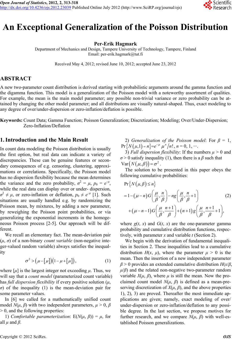