 Open Journal of Statistics, 2012, 2, 260-268 http://dx.doi.org/10.4236/ojs.2012.23031 Published Online July 2012 (http://www.SciRP.org/journal/ojs) An Empirical Bayes Approach to Robust Variance Estimation: A Statistical Proposal for Quantitative Medical Image Testing Zhan-Qian John Lu1,2, Charles Fenimore1, Ronald H. Gottlieb3, Carl C. Jaffe4 1National Institute of Standards and Technology, Gaithersburg, USA 2Statistical Engineering Division (776), Information Technology Laboratory, NIST, Gaithersburg, USA 3University of Arizona, Tucson, USA 4Boston University, Boston, USA Email: john.lu@nist.gov Received March 30, 2012; revised May 2, 2012; accepted May 12, 2012 ABSTRACT The current standard for measuring tumor response using X-ray, CT and MRI is based on the response evaluation crite- rion in solid tumors (RECIST) which, while providing simplifications over previous (WHO) 2-D methods, stipulate four response categories: CR (complete response), PR (partial response), PD (progressive disease), SD (stable disease) based purely on percentage changes without consideration of any measurement uncertainty. In this paper, we propose a statistical procedure for tumor response assessment based on uncertainty measures of radiologist’s measurement data. We present several variance estimation methods using time series methods and empirical Bayes methods when a small number of serial observations are available on each member of a group of subjects. We use a publically available data- base which contains a set of over 100 CT scan images on 23 patients with annotated RECIST measurements by two radiologist readers. We show that despite the bias in each individual reader’s measurements, statistical decisions on tu- mor change can be made on each individual subject. The consistency of the two readers can be established based on the intra-reader change assessments. Our proposal compares favorably with the RECIST standard protocol, raising the hope that, statistically sound decision on change analysis can be made in the future based on careful variability and meas- urement uncertainty analysis. Keywords: RECIST; Quantitative Imaging as a Biomarker; Change Analysis; Lung CT Image Measurement; Inter-Reader and Intra-Reader Variability; Time Series Variance Estimation; Estimation of Many Variances; Statistical Decision Rule on Change 1. Introduction Currently there is much interest in treating quantitative medical imaging as a biomarker, employing medical im- aging tools to assess tumor change, especially in the as- sessment of response to medical therapy. In order to use medical imaging effectively as quantitative measurement tools, a number of questions are raised regarding quanti- fying cancerous tumor changes over course of time, such as What measures should be used in quantifying mean- ingful change or response of suspicious tumor objects from images, whether it is based on volume (3D) which has attracted a lot of current interest, or the WHO1 (2D) or RECIST (1D) [1,2]? What is the basic variability in these measures, in- cluding both intrinsic measurement variability (e.g. repeatability and reproducibility, and effects from dif- ferent instrument settings), and expert bias in marking up these measures, or biological variability? A critical but related question is—given the variabil- ity in imaging acquisition analysis, what is the mini- mum change that can be detected for a given imaging modality and a chosen image processing method and sizing measure. For example, one would like to know with credible statistical accuracy how large a meas- ured size change must be in order to be declared “sig- nificant” in a single individual? In this paper, we present preliminary steps toward a statistical methodology for variance estimation that will help address these questions. Because there are typically few measurements available on each individual subject, even in a longitudinal study, it is crucial that individual variance estimates for many patients be pooled together 1Acronym for the World Health Organization tumor measurement technique which assesses size change over time based on two or- thogonal dimensions of the objec . C opyright © 2012 SciRes. OJS 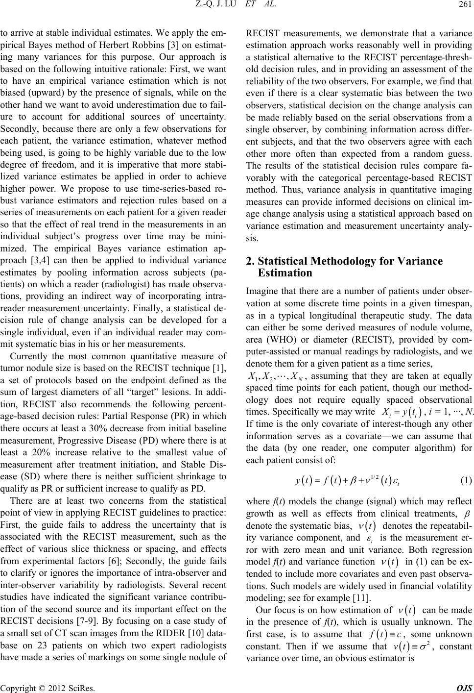 Z.-Q. J. LU ET AL. 261 to arrive at stable individual estimates. We apply the em- pirical Bayes method of Herbert Robbins [3] on estimat- ing many variances for this purpose. Our approach is based on the following intuitive rationale: First, we want to have an empirical variance estimation which is not biased (upward) by the presence of signals, while on the other hand we want to avoid underestimation due to fail- ure to account for additional sources of uncertainty. Secondly, because there are only a few observations for each patient, the variance estimation, whatever method being used, is going to be highly variable due to the low degree of freedom, and it is imperative that more stabi- lized variance estimates be applied in order to achieve higher power. We propose to use time-series-based ro- bust variance estimators and rejection rules based on a series of measurements on each patient for a given reader so that the effect of real trend in the measurements in an individual subject’s progress over time may be mini- mized. The empirical Bayes variance estimation ap- proach [3,4] can then be applied to individual variance estimates by pooling information across subjects (pa- tients) on which a reader (radiologist) has made observa- tions, providing an indirect way of incorporating intra- reader measurement uncertainty. Finally, a statistical de- cision rule of change analysis can be developed for a single individual, even if an individual reader may com- mit systematic bias in his or her measurements. Currently the most common quantitative measure of tumor nodule size is based on the RECIST technique [1], a set of protocols based on the endpoint defined as the sum of largest diameters of all “target” lesions. In addi- tion, RECIST also recommends the following percent- age-based decision rules: Partial Response (PR) in which there occurs at least a 30% decrease from initial baseline measurement, Progressive Disease (PD) where there is at least a 20% increase relative to the smallest value of measurement after treatment initiation, and Stable Dis- ease (SD) where there is neither sufficient shrinkage to qualify as PR or sufficient increase to qualify as PD. There are at least two concerns from the statistical point of view in applying RECIST guidelines to practice: First, the guide fails to address the uncertainty that is associated with the RECIST measurement, such as the effect of various slice thickness or spacing, and effects from experimental factors [6]; Secondly, the guide fails to clarify or ignores the importance of intra-observer and inter-observer variability by radiologists. Several recent studies have indicated the significant variance contribu- tion of the second source and its important effect on the RECIST decisions [7-9]. By focusing on a case study of a small set of CT scan images from the RIDER [10] data- base on 23 patients on which two expert radiologists have made a series of markings on some single nodule of RECIST measurements, we demonstrate that a variance estimation approach works reasonably well in providing a statistical alternative to the RECIST percentage-thresh- old decision rules, and in providing an assessment of the reliability of the two observers. For example, we find that even if there is a clear systematic bias between the two observers, statistical decision on the change analysis can be made reliably based on the serial observations from a single observer, by combining information across differ- ent subjects, and that the two observers agree with each other more often than expected from a random guess. The results of the statistical decision rules compare fa- vorably with the categorical percentage-based RECIST method. Thus, variance analysis in quantitative imaging measures can provide informed decisions on clinical im- age change analysis using a statistical approach based on variance estimation and measurement uncertainty analy- sis. 2. Statistical Methodology for Variance Estimation Imagine that there are a number of patients under obser- vation at some discrete time points in a given timespan, as in a typical longitudinal therapeutic study. The data can either be some derived measures of nodule volume, area (WHO) or diameter (RECIST), provided by com- puter-assisted or manual readings by radiologists, and we denote them for a given patient as a time series, 12 ,,, XX , assuming that they are taken at equally spaced time points for each patient, though our method- ology does not require equally spaced observational times. Specifically we may write ii yt, i = 1, ···, N. If time is the only covariate of interest-though any other information serves as a covariate—we can assume that the data (by one reader, one computer algorithm) for each patient consist of: 1/2 t ytf tt (1) where f(t) models the change (signal) which may reflect growth as well as effects from clinical treatments, denote the systematic bias, denotes the repeatabil- ity variance component, and t t is the measurement er- ror with zero mean and unit variance. Both regression model f(t) and variance function in (1) can be ex- tended to include more covariates and even past observa- tions. Such models are widely used in financial volatility modeling; see for example [11]. t t Our focus is on how estimation of can be made in the presence of f(t), which is usually unknown. The first case, is to assume that tc 2 vt , some unknown constant. Then if we assume that , constant variance over time, an obvious estimator is Copyright © 2012 SciRes. OJS 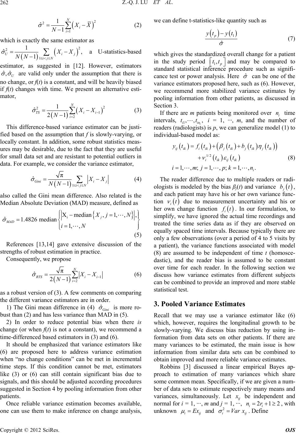 Z.-Q. J. LU ET AL. 262 21 ˆ1 2 1 N i i X N (2) which is exactly the same estimator as 2, ij N XX ˆˆ ,U 2 1 1 ˆ1 U ij NN a U-statistics-based estimator, as suggested in [12]. However, estimators are valid only under the assumption that there is no change, or f(t) is a constant, and will be heavily biased if f(t) changes with time. We present an alternative esti- mator, 2 1 i i XX 2 2 1 ˆ21 N TS i N (3) This difference-based variance estimator can be justi- fied based on the assumption that f is slowly-varying, or locally constant. In addition, some robust statistics meas- ures may be desirable, due to the fact that they are useful for small data set and are resistant to potential outliers in data. For example, we consider the variance estimator, 1 π ˆ1 Ginii j ijN X NN (4) also called the Gini mean difference. Also related is the Median Absolute Deviation (MAD) measure, defined as i Xmedian , ˆ1.4826 median 1, , j MAD Xj iN 1,, ,N (5) References [13,14] gave extensive discussion of the strengths of robust estimation in practice. Consequently, we propose 1 2 N π ˆ21 TSi i i X ˆ N (6) as a robust version of (3). A few comments on comparing the different variance estimators are in order. 1) The Gini mean difference in (4) Gini is more ro- bust than (2) and has less variance than MAD in (5). 2) In order to reduce potential bias when there is change (or when f(t) is not a constant), we recommend a time-differenced based estimators in (3) and (6). It should be emphasized that variance estimators like (6) are proposed here to address variance estimation when “no change conditions” can be met in incremental time steps. If this condition cannot be met, estimators like (3) or (6) can still contain significant bias due to signals, and this should be adjusted according procedures suggested in Section 4 by pooling information from other patients. Once reliable variance estimation becomes available, one can use them to make inference on change analysis, we can define t-statistics-like quantity such as 1 ˆ p yt yt , (7) which gives the standardized overall change for a patient in the study period 1 tt and may be compared to standard statistical inference procedure such as signifi- cance test or power analysis. Here ˆ can be one of the variance estimators proposed here, such as (6). However, we recommend more stabilized variance estimates by pooling information from other patients, as discussed in Section 3. If there are m patients being monitored over i time intervals, 1i iin i = 1, ···, m, and the number of readers (radiologists) is p, we can generalize model (1) to individual-based model as: n ,,,tt 1/2 1, ,;1, ,;1, ,. ij iki ikj ikj ikj ik iikijik i tfttbt t tt imj pkn (8) The reader difference due to multiple readers or radi- ologists is modeled by the bias βj(t) and variance bt j, and each patient may have his or her own variance func- tion t i due to measurement uncertainty and his or her own change function i t. In our formulation, to simplify, we have ignored the actual time recordings and treated the time series data as if they are observed on equally spaced time intervals. Because typically there are only a few observations (over a period of 4 to 5 visits by a patient), the variance functions associated with model (8) are assumed to be independent of time t (homosce- dastic), and the reader bias is assumed to be constant over time for each reader. In the following section we discuss how variance estimates from different subjects can be combined to provide an improved and more stable statistical test. 3. Pooled Variance Estimates Recall that we may use a variance estimator like (6) which, however, requires the longitudinal growth to be slowly-varying. We discuss bias reduction by using in- formation from data sets on other patients. If there are many variances to be estimated, the main issue is how information from similar data sets can be combined to obtain improved and more reliable variance estimates. Robbins [3] discussed a linear empirical Bayes ap- proach to estimation of many variances which share some common mean. Specifically, if we are given a num- ber of data sets to estimate respectively many means and variances, simultaneously. Let ij be independent and normal for i = 1, ···, m and j = 1, ···, ii, with unknown 212nr iij Ex and . Define 2 iij Var x Copyright © 2012 SciRes. OJS 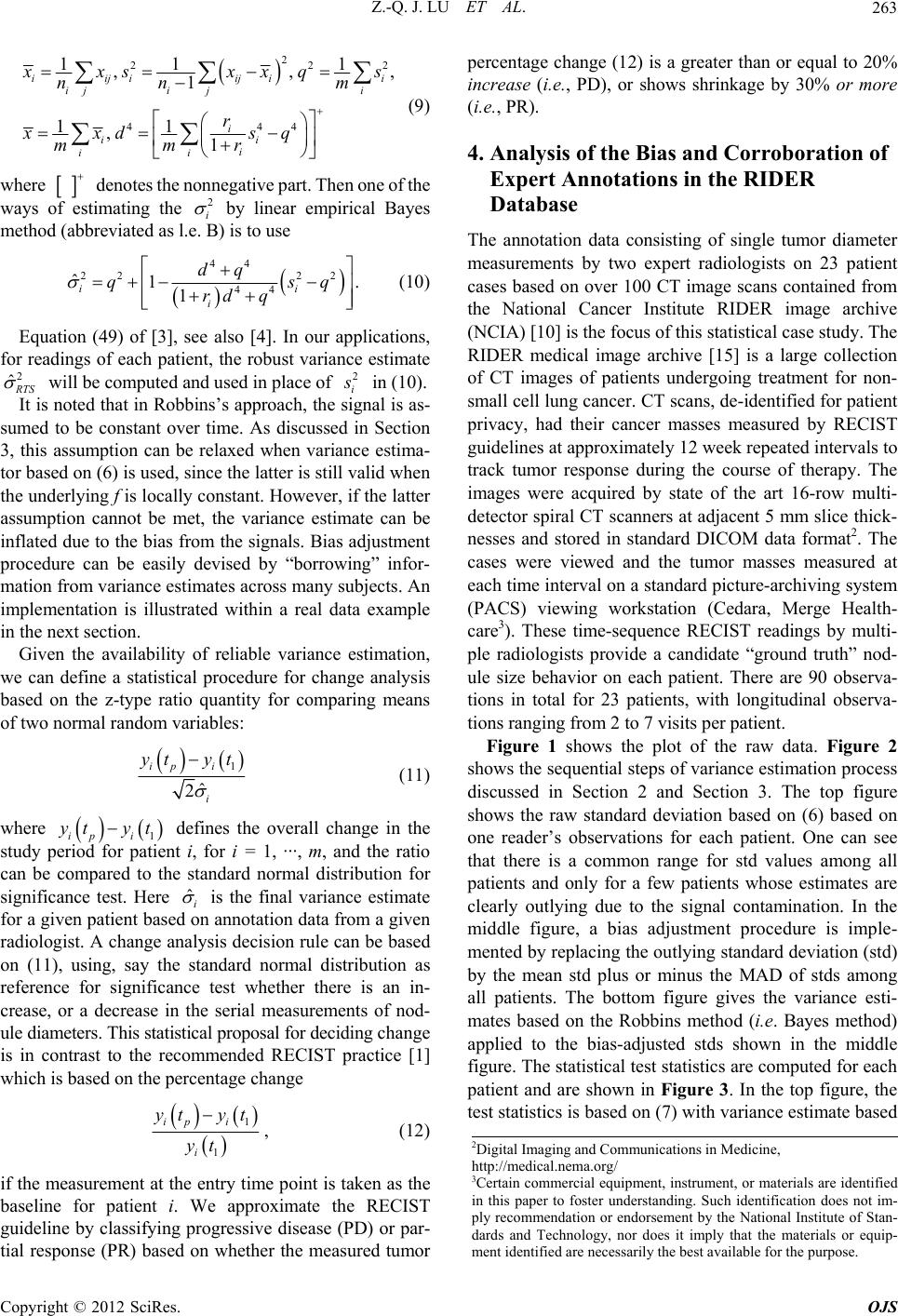 Z.-Q. J. LU ET AL. 263 2 2 44 11 ,, 1 11 ,1 iijiij ii jj i ii i ii 2 2 4 1 , i i i xsx x nn r xxd s mmr q s m q 2 (9) where denotes the nonnegative part. Then one of the ways of estimating the i by linear empirical Bayes method (abbreviated as l.e. B) is to use 22 44 1 ii i dq qsq rd q 2 ˆ 44 22 ˆ1. (10) Equation (49) of [3], see also [4]. In our applications, for readings of each patient, the robust variance estimate TS will be computed and used in place of 2 i in (10). It is noted that in Robbins’s approach, the signal is as- sumed to be constant over time. As discussed in Section 3, this assumption can be relaxed when variance estima- tor based on (6) is used, since the latter is still valid when the underlying f is locally constant. However, if the latter assumption cannot be met, the variance estimate can be inflated due to the bias from the signals. Bias adjustment procedure can be easily devised by “borrowing” infor- mation from variance estimates across many subjects. An implementation is illustrated within a real data example in the next section. Given the availability of reliable variance estimation, we can define a statistical procedure for change analysis based on the z-type ratio quantity for comparing means of two normal random variables: 1 ˆ 2 ip i i yt yt yt yt ˆ (11) where 1ipi defines the overall change in the study period for patient i, for i = 1, ···, m, and the ratio can be compared to the standard normal distribution for significance test. Here i is the final variance estimate for a given patient based on annotation data from a given radiologist. A change analysis decision rule can be based on (11), using, say the standard normal distribution as reference for significance test whether there is an in- crease, or a decrease in the serial measurements of nod- ule diameters. This statistical proposal for deciding change is in contrast to the recommended RECIST practice [1] which is based on the percentage change 1 1 ip i i yt yt yt , (12) if the measurement at the entry time point is taken as the baseline for patient i. We approximate the RECIST guideline by classifying progressive disease (PD) or par- tial response (PR) based on whether the measured tumor percentage change (12) is a greater than or equal to 20% increase (i.e., PD), or shows shrinkage by 30% or more (i.e., PR). 4. Analysis of the Bias and Corroboration of Expert Annotations in the RIDER Database The annotation data consisting of single tumor diameter measurements by two expert radiologists on 23 patient cases based on over 100 CT image scans contained from the National Cancer Institute RIDER image archive (NCIA) [10] is the focus of this statistical case study. The RIDER medical image archive [15] is a large collection of CT images of patients undergoing treatment for non- small cell lung cancer. CT scans, de-identified for patient privacy, had their cancer masses measured by RECIST guidelines at approximately 12 week repeated intervals to track tumor response during the course of therapy. The images were acquired by state of the art 16-row multi- detector spiral CT scanners at adjacent 5 mm slice thick- nesses and stored in standard DICOM data format2. The cases were viewed and the tumor masses measured at each time interval on a standard picture-archiving system (PACS) viewing workstation (Cedara, Merge Health- care3). These time-sequence RECIST readings by multi- ple radiologists provide a candidate “ground truth” nod- ule size behavior on each patient. There are 90 observa- tions in total for 23 patients, with longitudinal observa- tions ranging from 2 to 7 visits per patient. Figure 1 shows the plot of the raw data. Figure 2 shows the sequential steps of variance estimation process discussed in Section 2 and Section 3. The top figure shows the raw standard deviation based on (6) based on one reader’s observations for each patient. One can see that there is a common range for std values among all patients and only for a few patients whose estimates are clearly outlying due to the signal contamination. In the middle figure, a bias adjustment procedure is imple- mented by replacing the outlying standard deviation (std) by the mean std plus or minus the MAD of stds among all patients. The bottom figure gives the variance esti- mates based on the Robbins method (i.e. Bayes method) applied to the bias-adjusted stds shown in the middle figure. The statistical test statistics are computed for each patient and are shown in Figure 3. In the top figure, the test statistics is based on (7) with variance estimate based 2Digital Imaging and Communications in Medicine, http://medical.nema.org/ 3Certain commercial equipment, instrument, or materials are identified in this paper to foster understanding. Such identification does not im- ly recommendation or endorsement by the National Institute of Stan- dards and Technology, nor does it imply that the materials or equip- ment identified are necessarily the best available for the purpose. Copyright © 2012 SciRes. OJS 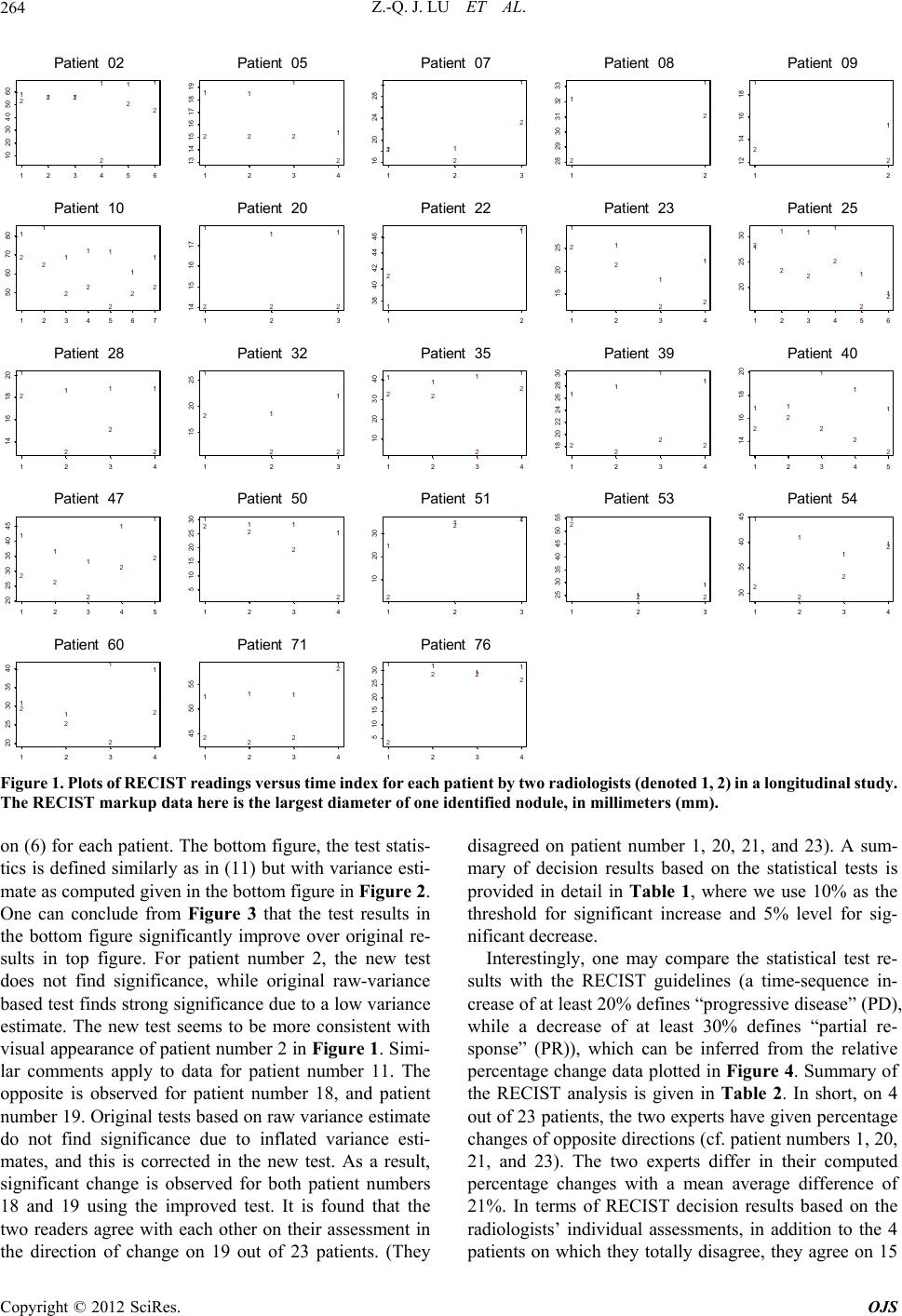 Z.-Q. J. LU ET AL. Copyright © 2012 SciRes. OJS 264 111 111 222 2 22 123456 10 20 30 40 50 60 Patient 02 11 1 1 222 2 1234 13 14 15 16171819 Patient 05 11 1 2 2 2 123 16 20 24 28 Patient 07 1 1 2 2 12 28 29 30 31 32 33 Patient 08 1 2 1 2 12 12 14 16 18 P 11 111 1 12 2 22 2 22 at ient 09 1234567 50 60 70 80 Patient 10 111 222 123 14 1516 17 Patient 20 1 1 2 2 12 38 40 42 44 46 Patient 22 1 1 1 1 2 2 22 1234 15 20 25 Patient 23 1 1 2 2 11 1 1 2 2 2 2 123456 20 25 30 P 1 111 2 2 2 2 at ient 25 1234 14 1618 20 Patient 28 1 1 1 2 22 123 15 20 25 Patient 32 1111 22 2 2 1234 10 20 30 40 Patient 35 11 11 22 22 1234 18 20 22 24 262830 Patient 39 11 2 2 1 1 1 2 2 2 12345 14 16 18 20 P 1 1 1 11 22 2 22 at ient 40 12345 20 25 30 35 40 45 Patient 47 1111 22 2 2 1234 5 1015202530 Patient 50 1 11 2 22 123 10 20 30 Patient 51 1 1 1 2 22 123 25 30 35 40 45 50 55 Patient 53 1 2 1 1 1 2 2 2 1234 30 35 40 45 P 1 1 11 2 2 2 2 at ient 54 1234 20 25 3035 40 Patient 60 111 1 222 2 1234 45 50 55 Patient 71 1111 2 222 1234 5 1015202530 Patient 76 Figure 1. Plots of RECIST readings versus time index for each patient b y two radiologists (denoted 1, 2) in a longitudinal st udy. The RECIST markup data here is the largest diameter of one identified nodule, in millimeters (mm). on (6) for each patient. The bottom figure, the test statis- tics is defined similarly as in (11) but with variance esti- mate as computed given in the bottom figure in Figure 2. One can conclude from Figure 3 that the test results in the bottom figure significantly improve over original re- sults in top figure. For patient number 2, the new test does not find significance, while original raw-variance based test finds strong significance due to a low variance estimate. The new test seems to be more consistent with visual appearance of patient number 2 in Figure 1. Simi- lar comments apply to data for patient number 11. The opposite is observed for patient number 18, and patient number 19. Original tests based on raw variance estimate do not find significance due to inflated variance esti- mates, and this is corrected in the new test. As a result, significant change is observed for both patient numbers 18 and 19 using the improved test. It is found that the two readers agree with each other on their assessment in the direction of change on 19 out of 23 patients. (They disagreed on patient number 1, 20, 21, and 23). A sum- mary of decision results based on the statistical tests is provided in detail in Table 1, where we use 10% as the threshold for significant increase and 5% level for sig- nificant decrease. Interestingly, one may compare the statistical test re- sults with the RECIST guidelines (a time-sequence in- crease of at least 20% defines “progressive disease” (PD), while a decrease of at least 30% defines “partial re- sponse” (PR)), which can be inferred from the relative percentage change data plotted in Figure 4. Summary of the RECIST analysis is given in Table 2. In short, on 4 out of 23 patients, the two experts have given percentage changes of opposite directions (cf. patient numbers 1, 20, 21, and 23). The two experts differ in their computed percentage changes with a mean average difference of 21%. In terms of RECIST decision results based on the radiologists’ individual assessments, in addition to the 4 patients on which they totally disagree, they agree on 15 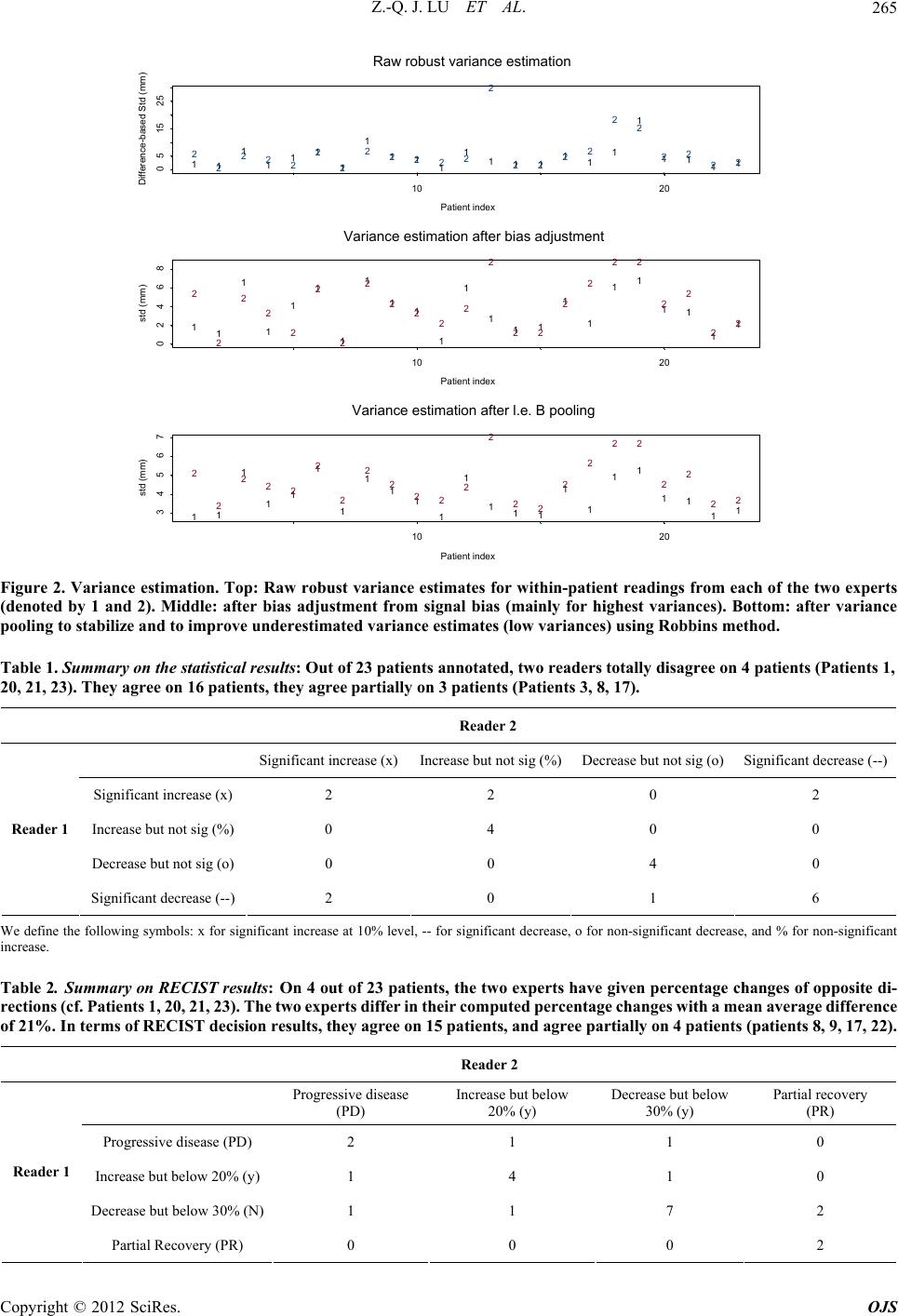 Z.-Q. J. LU ET AL. 265 11 1 111 1 1 111 1111111 1 1 2 2 222 2 2 22222 2 2222 22 2 Patient index Difference-based Std (mm) 111 222 10 20 0 51525 Raw robust variance estimati on 11 1 1 1 1 1 1 11 1 1 111 1 1 11 1 2 2 2 2 2 2 2 2 222 2 2 22 2 2 22 2 Patient index std (mm) 1 11 2 22 10 20 02468 Variance estimation after bias adjustment 11 1 11 1 1 111 1 1 111 1 1 11 1 2 2 222 2 2 2 222 2 2 22 2 2 22 2 Patient index std (mm) 1 11 2 22 10 20 34567 Variance estimation after l.e. B pooling Figure 2. Variance estimation. Top: Raw robust variance estimates for within-patient readings from each of the two experts (denoted by 1 and 2). Middle: after bias adjustment from signal bias (mainly for highest variances). Bottom: after variance pooling to stabilize and to improve underestimated variance estimates (low variances) using Robbins method. Table 1. Summary on the statistical results: Out of 23 patients annotated, two readers totally disagree on 4 patients (Patients 1, 20, 21, 23). They agree on 16 patients, they agree partially on 3 patients (Patients 3, 8, 17). Reader 2 Significant increase (x)Increase but not sig (%)Decrease but not sig (o) Significant decrease (--) Significant increase (x)2 2 0 2 Increase but not sig (%)0 4 0 0 Decrease but not sig (o)0 0 4 0 Reader 1 Significant decrease (--)2 0 1 6 We define the following symbols: x for significant increase at 10% level, -- for significant decrease, o for non-significant decrease, and % for non-significant increase. Table 2. Summary on RECIST results: On 4 out of 23 patients, the two experts have given percentage changes of opposite di- rections (cf . Patients 1, 20, 21, 2 3). The two experts differ in their comp uted percen tage changes with a mean a verage differen ce of 21%. In terms of RECIST decision results, t hey agree on 15 patients, and agree partially on 4 patients (patients 8, 9, 17, 22). Reader 2 Progressive disease (PD) Increase but below 20% (y) Decrease but below 30% (y) Partial recovery (PR) Progressive disease (PD) 2 1 1 0 Increase but below 20% (y) 1 4 1 0 Decrease but below 30% (N) 1 1 7 2 Reader 1 Partial Recovery (PR) 0 0 0 2 Copyright © 2012 SciRes. OJS 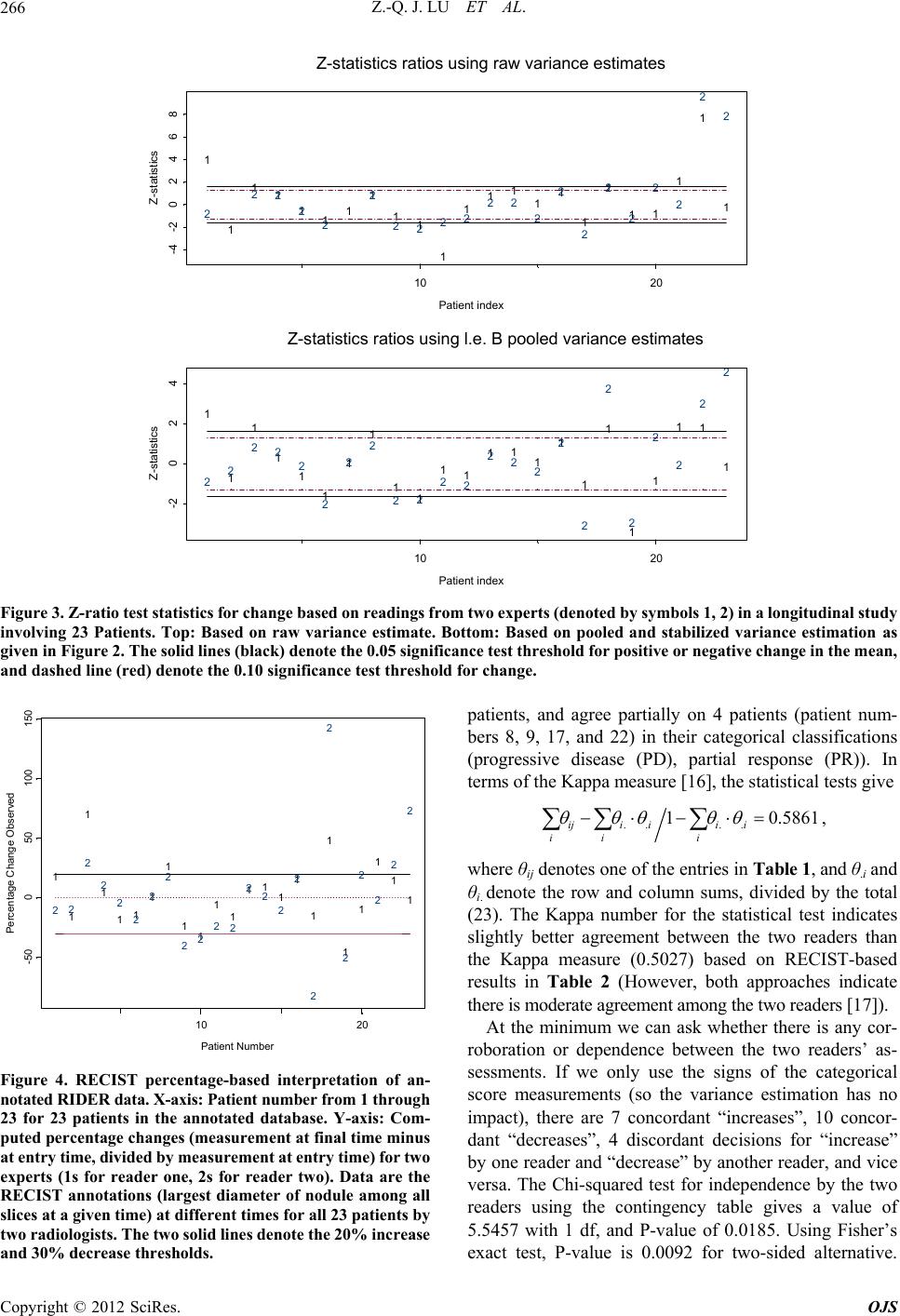 Z.-Q. J. LU ET AL. 266 1 1 111111 11 1 11111 1 1 1 2 2222 2 2222 222 2 2 2 2 Patient index Z-statistics 1 1 1 1 2 2 2 2 10 20 -4-202468 Z-statistics ratios using raw variance estimates 1 1 1 1 1 1 1 1 11 11 111 1 1 1 1 22 222 2 2 2 22 22 222 2 2 2 2 Patient index Z-statistics 1 11 1 2 2 2 2 10 20 -2 024 Z-statistics ratios using l.e. B pooled variance estimates Figure 3. Z -ratio test s tatistics f or chan ge base d on read ings from t wo experts (denoted by symbols 1, 2) in a longitudinal study involving 23 Patients. Top: Based on raw variance estimate. Bottom: Based on pooled and stabilized variance estimation as given in Figure 2. The solid lines (black) denote the 0.05 significance test threshold for positive or negative change in the mean, and dashed line (red) denote the 0.10 significance test threshold for change. 1 1 1 1 11 1 1 11 11 111 1 1 22 2 2 2 2 2 2 2222 222 2 2 Patient Number Percentage Change Observed 1 1 1 1 1 1 2 2 2 2 2 2 10 20 -50050100 150 Figure 4. RECIST percentage-based interpretation of an- notated RIDER data. X-axis: Patient number from 1 through 23 for 23 patients in the annotated database. Y-axis: Com- puted percentage changes (measurement at final time minus at entry time, divided by measurement at entry time) for t wo experts (1s for reader one, 2s for reader two). Data are the RECIST annotations (largest diameter of nodule among all slices at a given time) at different times for all 23 patients by two radiologists. The two sol id lin es denote the 20% increas e and 30% decrease thresholds. patients, and agree partially on 4 patients (patient num- bers 8, 9, 17, and 22) in their categorical classifications (progressive disease (PD), partial response (PR)). In terms of the Kappa measure [16], the statistical tests give .. .. 1 0.5861 ij iiii ii i , where θij denotes one of the entries in Table 1, and θ.i and θi. denote the row and column sums, divided by the total (23). The Kappa number for the statistical test indicates slightly better agreement between the two readers than the Kappa measure (0.5027) based on RECIST-based results in Table 2 (However, both approaches indicate there is moderate agreement among the two readers [17]). At the minimum we can ask whether there is any cor- roboration or dependence between the two readers’ as- sessments. If we only use the signs of the categorical score measurements (so the variance estimation has no impact), there are 7 concordant “increases”, 10 concor- dant “decreases”, 4 discordant decisions for “increase” by one reader and “decrease” by another reader, and vice versa. The Chi-squared test for independence by the two readers using the contingency table gives a value of 5.5457 with 1 df, and P-value of 0.0185. Using Fisher’s exact test, P-value is 0.0092 for two-sided alternative. Copyright © 2012 SciRes. OJS 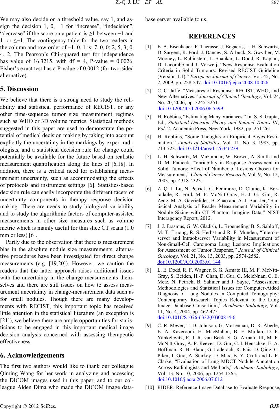 Z.-Q. J. LU ET AL. 267 We may also decide on a threshold value, say 1, and as- sign the decision 1, 0, −1 for “increase”, “indecision”, “decrease” if the score on a patient is ≥1 between −1 and 1, or ≤−1. The contingency table for the two readers in the column and row order of −1, 0, 1 is: 7, 0, 0; 2, 5, 3; 0, 4, 2. The Pearson’s Chi-squared test for independence has value of 16.3215, with df = 4, P-value = 0.0026. Fisher’s exact test has a P-value of 0.0012 (for two-sided alternative). 5. Discussion We believe that there is a strong need to study the reli- ability and statistical performance of RECIST, or any other time-sequence tumor size measurement regimes such as WHO or 3D volume metrics. Statistical methods suggested in this paper are used to demonstrate the po- tential of medical decision making by taking into account explicitly the uncertainty in the markings by expert radi- ologists, and a statistical decision rule for change could potentially be available for the future based on realistic measurement quantification along the lines of [6,18]. In addition, there is a critical need for establishing meas- urement uncertainty, such as accommodating the effects of protocols and instrument settings [6]. Statistics-based decision rule can easily incorporate the different facets of uncertainty components in therapy response decision making. There are needs to study biological variability and to study the algorithmic factors of computer-assisted measurements in other size measures such as volume metric which is mainly useful for thin slice CT scans (1.0 mm or less) [6]. Partly due to the observation that there is measurement bias in the absolute nodule size measurements, alterna- tive procedures have been investigated for direct change measurements (e.g. [19,20]). However, we caution the readers that the latter approach raises additional issues with the uncertainty in the change measurements them- selves and there are still issues on how to assess meas- urement uncertainty in change-measurement data such as for small nodules. Though there are many develop- ments with RECIST, this important topic has received little attention in the statistical literature (an exception is [21]), we believe there are ample opportunities for statis- ticians to be engaged in this important medical image decision analysis concerned with assessing therapeutic effectiveness. 6. Acknowledgements The first two authors would like to thank our colleague Qiming Wang for her work in analyzing and accessing the DICOM images used in this paper, and to our col- league Alden Dima who made the DICOM image data- base server available to us. REFERENCES [1] E. A. Eisenhauer, P. Therasse, J. Bogaerts, L. H. Schwartz, D. Sargent, R. Ford, J. Dancey, S. Arbuck, S. Gwyther, M. Mooney, L. Rubinstein, L. Shankar, L. Dodd, R. Kaplan, D. Lacombe and J. Verweij, “New Response Evaluation Criteria in Solid Tumours: Revised RECIST Guideline (Version 1.1),” European Journal of Cancer, Vol. 45, No. 2, 2009, pp. 228-247. doi:10.1016/j.ejca.2008.10.026 [2] C. C. Jaffe, “Measures of Response: RECIST, WHO, and New Alternatives,” Journal of Clinical Oncology, Vol. 24, No. 20, 2006, pp. 3245-3251. doi:10.1200/JCO.2006.06.5599 [3] H. Robbins, “Estimating Many Variances,” In: S. S. Gupta, Ed., Statistical Decision Theory and Related Topics III, Vol. 2, Academic Press, New York, 1982, pp. 251-261. [4] H. Robbins, “Some Thoughts on Empirical Bayes Eesti- mation,” Annals of Statistics, Vol. 11, No. 3, 1983, pp. 713-723. doi:10.1214/aos/1176346239 [5] L. H. Schwartz, M. Mazumdar, W. Brown, A. Smith and D. M. Panicek, “Variability in Response Assessment in Solid Tumors: Effect of Number of Lesions Chosen for Measurement,” Clinical Cancer Research, Vol. 9, No. 12, 2003, pp. 4318-4323. [6] Z. Q. J. Lu, N. Petrick, C. Fenimore, D. Clunie, K. Bor- radaile, R. Ford, M. F. McNitt-Gray, H. J. G. Kim, R. Zeng, M. A. Gavrielides, B. Zhao and A. J. Buckler, “Sta- tistical Analysis of Reader Measurement Variability in Nodule Sizing with CT Phantom Imaging Data,” NIST Interagency Report, 2012. [7] J. J. Erasmus, G. W. Gladish, L. Broemeling, B. S. Sabloff, M. T. Truong, R. S. Herbst and R. F. Munden, “Interob- server and Intraobserver Variability in Measurement of Non-Small-Cell Carcinoma Lung Lesions: Implications for Assessment of Tumor Response,” Journal of Clinical Oncology, Vol. 21, No. 13, 2003, pp. 2574-2582. doi:10.1200/JCO.2003.01.144 [8] L. E. Dodd, R. F. Wagner, S. G. Armato III, M. F. McNitt- Gray, S. Beiden, H.-P. Chan, D. Gur, G. McleNnan, C. E. Metz, N. Petrick, B. Sahiner and J. Sayre, “Assessment Methodologies and Statistical Issues for Computer-Aided Diagnosis of Lung Nodules in Computed Tomography: Contemporary Research Topics Relevant to the Lung Image Database Consortium,” Academic Radiology, Vol. 11, No. 4, 2004, pp. 462-475. doi:10.1016/S1076-6332(03)00814-6 [9] C. R. Meyer, T. D. Johnson, G. McLennan, D. R. Aberle, E. A. Kazerooni, H. MacMahon, B. F. Mullan, D. F. Yankelevitz, E. J. R. van Beek, S. G. Armato III, M. F. McNitt-Gray, A. P. Reeves, D. Gur, C. I. Henschke, E. A. Hoffman, R. H. Bland, G. Laderach, R. Pais, D. Qing, C. Piker, J. Guo, A. Starkey, D. Max, B. Y. Croft and L. P. Clarke, “Evaluation of Lung MDCT Nodule Annotation Across Radiologists and Methods,” Academic Radiology, Vol. 13, No. 10, 2006, pp. 1254-1265. doi:10.1016/j.acra.2006.07.012 [10] RIDER: Reference Image Database to Evaluate Response, Copyright © 2012 SciRes. OJS  Z.-Q. J. LU ET AL. Copyright © 2012 SciRes. OJS 268 National Institute of Biomedical Imaging and Bioengi- neering Institute of NIH. http://www.nibib.nih.gov/Research/Resources/ImageClin Data#RIDER [11] Z. Q. Lu, “Local Polynomial Prediction and Volatility Estimation in Financial Time Series,” In: A. S. Soofi and L. Cao, Eds., Modelling and Forecasting Financial Data: Techniques of Nonlinear Dynamics, Kluwer, Boston, 2002, pp. 115-135. [12] C. R. Meyer, S. G. Armato III, C. P. Fenimore, G. McLen- nan, L. M. Bidaut, D. P. Barboriak, M. A. Gavrielides, E. F. Jackson, M. F. McNitt-Gray, P. E. Kinahan, N. Petrick and B. Zhao, “Quantitative Imaging to Assess Tumor Response to Therapy: Common Themes of Measurement, Truth Data, and Error Sources,” Translational Oncology, Vol. 2, No. 4, 2009, pp.198-210. [13] P. J. Huber, “Robust Statistics,” Wiley, New York, 1981. [14] D. C. Hoaglin, F. Mosteller and J. W. Tukey, “Under- standing Robust and Exploratory Data Analysis,” Wiley, New York, 1983. [15] S. G. Armato III, C. R. Meyer, M. F. McNitt-Gray, G. McLennan, A. P. Reeves, B. Y. Croft and L. P. Clarke, “The Reference Image Database to Evaluate Response to Therapy in Lung Cancer (RIDER) Project: A Resource for the Development of Change-Analysis Software,” Clinical Pharmacology & Therapeutics, Vol. 84, No. 4, 2008, pp. 448-456. doi:10.1038/clpt.2008.161 [16] J. R. Landis and G. G. Koch, “The Measurement of Ob- server Agreement for Categorical Data,” Biometrics, Vol. 33, No. 1, 1977, pp. 159-174. doi:10.2307/2529310 [17] A. J. Viera and J. M. Garrett, “Understanding the In- terobserver Agreement: The Kappa Statistics,” Family Medicine, Vol. 37, No. 5, 2005, pp. 360-363. [18] B. Zhao, L. P. James, C. S. Moskowitz, P. Guo, M. S. Ginsberg, R. A. Lefkowitz, Y. Qin, G. J. Riely, M. G. Kris and L. H. Schwartz, “Evaluating Variability in Tu- mor Measurements from Same-Day Repeat Scans of Pa- tients with Non-Small Cell Lung Cancer,” Radiology, Vol. 252, No. 1, 2009, pp. 263-272. doi:10.1148/radiol.2522081593 [19] A. P. Reeves, A. B. Chan, D. F. Yankelevitz, C. I. Hen- schke, B. Kressler, W. J. Kostis, “On Measuring the Change in Size of Pulmonary Nodules,” IEEE Transac- tions on Medical Imaging, Vol. 25, No. 4, 2006, pp. 435- 450. doi:10.1109/TMI.2006.871548 [20] J. M. Reinhardt, K. Ding, K. Cao, C. E. Christensen, E. A. Hoffman and S. V. Bodas, “Registration-Based Estimates of Local Lung Tissue Expansion Compared to Xenon CT Measures of Specific Ventilation,” Medical Image Analy- sis, Vol. 12, No. 6, 2008, pp. 752-763. doi:10.1016/j.media.2008.03.007 [21] L. D. Broemeling, “Bayesian Biostatistics and Diagnostic Medicine,” Chapmall & Hll/CRC, Boca Raton, 2007.
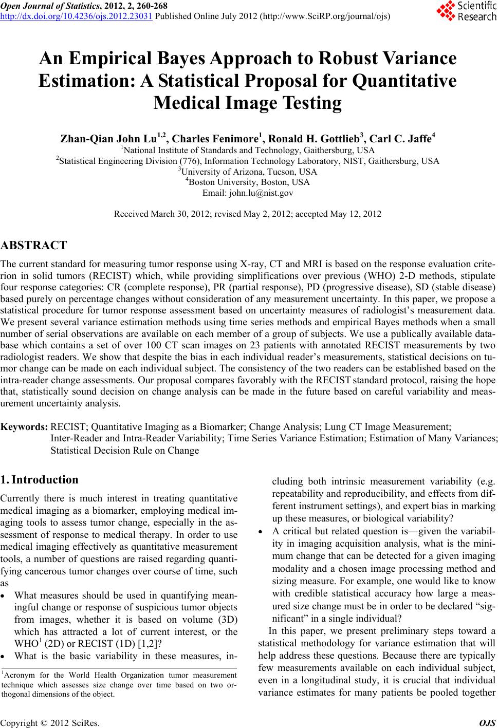
|