 Open Journal of Statistics, 2012, 2, 281-296 http://dx.doi.org/10.4236/ojs.2012.23034 Published Online July 2012 (http://www.SciRP.org/journal/ojs) Subsampling Method for Robust Estimation of Regression Models Min Tsao, Xiao Ling Department of Mathematics and Statistics, University of Victoria, Victoria, Canada Email: tsao@math.uvic.ca Received March 29, 2012; revised April 30, 2012; accepted May 10, 2012 ABSTRACT We propose a subsampling method for robust estimation of regression models which is built on classical methods such as the least squares method. It makes use of the non-robust nature of the underlying classical method to find a good sample from regression data contaminated with outliers, and then applies the classical method to the good sample to produce robust estimates of the regression model parameters. The subsampling method is a computational method rooted in the bootstrap methodology which trades analytical treatment for intensive computation; it finds the good sam- ple through repeated fitting of the regression model to many random subsamples of the contaminated data instead of through an analytical treatment of the outliers. The subsampling method can be applied to all regression models for which non-robust classical methods are available. In the present paper, we focus on the basic formulation and robust- ness property of the subsampling method that are valid for all regression models. We also discuss variations of the method and apply it to three examples involving three different regression models. Keywords: Subsampling Algorithm; Robust Regression; Outliers; Bootstrap; Goodness-of-Fit 1. Introduction Robust estimation and inference for regression models is an important problem with a long history in robust statistics. Earlier work on this problem is discussed in [1] and [2]. The first book focusing on robust regression is [3] which gives a thorough coverage of robust regression methods developed prior to 1987. There have been many new developments in the last two decades. Reference [4] pro- vides a good coverage on many recent robust regression methods. Although there are now different robust methods for various regression models, most existing methods involve a quantitative measure of the outlyingness of individual observations which is used to formulate robust estimators. That is, contributions from individual observa- tions to the estimators are weighted depending on their degrees of outlyingness. This weighting by outlyingness is done either explicitly as in, for example, the GM- estimators of [5] or implicitly as in the MM-estimator of [6] through the use of functions. In this paper, we introduce an alternative method for robust regression which does not involve any explicit or implicit notion of outlyingness of individual observations. Our alternative method focuses instead on the presence or absence of outliers in a subset (subsample) of a sam- ple, which does not require a quantitative characteri- sation of outlyingness of individual observations, and attempts to identify the subsample which is free of out- liers. Our method makes use of standard non-robust classical regression methods for both identifying the outlier free subsamples and then estimating the regres- sion model with the outlier free subsamples. Specifically, suppose we have a sample consisting of mostly “good data points” from an ideal regression model and some outliers which are not generated by the ideal model, and we wish to estimate the ideal model. The basic idea of our method is to consider subsamples taken without re- placement from the contaminated sample and to identify, among possibly many subsamples, “good subsamples” which contain only good data points. Then estimate the ideal regression model using only the good subsamples through a simple classical method. The identification of good subsamples is accomplished through fitting the model to many subsamples with the classical method, and then using a criterion, typically a goodness-of-fit measure that is sensitive to the presence of outliers, to determine whether the subsamples contain outliers. We will refer to this method as the subsampling method. The subsampling method has three attractive aspects: 1) it is based on elements of classical methods, and as such it can be readily constructed to handle all regression models for which non-robust classical methods are available, 2) under certain conditions, it provides unbiased estimators for the ideal regression model parameters, and 3) it is C opyright © 2012 SciRes. OJS  M. TSAO, X. LING 282 =,, ii EY gx easy to implement as it does not involve the potentially difficult task of formulating the outlyningness of indi- vidual observations and their weighting. Point (3) above is particularly interesting as evaluating the outlyingness of individual observations is tradi- tionally at the heart of robust methods, yet in the re- gression context this task can be particularly difficult. To further illustrate this point, denote by an observation where i is the response and i the corresponding covariates vector. The outlyingness of obseravtion ii here is with respect to the under- lying regression model, not with respect to a fixed point in as is in the location problem. It may be an outlier due to the outlyingness in either i or i Y or both. In simple regression models where the underlying models have nice geometric representations, such as the linear or multiple linear regression models, the outlying- ness of an ii may be characterized by extending measures of outlyingness for the location problem through for example the residuals. But in cases where i is discrete such as a binary, Poisson or multinomial re- sponse, the geometry of the underlying models are com- plicated and the outlyingness of ii may be dif- ficult to formulate. With the subsampling methods, we avoid the need to formulate the outlyingness of indivi- dual observations but instead focus on the consequence of outliers, that is, they typically lead to a poor fit. We take advantage of this observation to remove the outliers and hence achieve robust estimation of regression models. It should be noted that traditionally the notion of an “outlier” is often associated with some underlying meas- ure of outlyingness of individual observations. In the present paper, however, by “outliers” we simply mean data points that are not generated by the ideal model and will lead to a poor fit. Consequently, the removal of outliers is based on the quality of fit of subsamples, not a measure of outlyingness of individual points. , ii YX 1 Yq X ,YX X ,YX Y =, ii 1q ,XY The rest of the paper is organized as follows. In Sec- tion 2, we set up notation and introduce the subsampling method. In Section 3, we discuss asymptotic and robust- ness properties of the subsampling estimator under general conditions not tied to a specific regression model. We then apply the subsampling methods to three examples involving three different regression models in Section 4. In Section 5, we discuss variations of the subsampling method which may improve the efficiency and reliability of the method. We conclude with a few remarks in Section 6. Proofs are given in the Appendix. 2. The Subsampling Method To set up notation, let i (1) where i 1 Y q iX 1 ,: q gxβ is the response variable, is the corresponding covariates vector, i is the regression function and β YX is the regression parameter vector. To accommodate different regression models, the distributions of i and i are left un- specified here. They are also not needed in our sub- sequent discussions. Denote by =,,, 12 N a contaminated sam- ple of observations containing “good data” ge- nerated by model (1) and “bad data” which are outliers not from the model. Here and m are un- known integers that add up to . Let n and m be the (unknown) partition of Szz z Nn m n N SS S S nSm such that n contains the good data and m contains the bad data. To achieve robust estimation of with S, the subsam- pling method first constructs a sample S n S to estimate the unknown good data set , and then applies a (non- robust) classical estimator to S. The resulting estimator for will be referred to as the subsampling estimator or SUE for . Clearly, a reliable and efficient S S S which captures a high percentage of the good data points in n but none of the bad points in m is the key to the robustness and the efficiency of the SUE. The subsampling algorithm that we develop below is aimed at generating a reliable and efficient S. 2.1. The Subsampling Algorithm be a random sample of size Let n taken without replacement from S, which we will refer to as a sub- sample of S. The key idea of the subsampling method is to construct the estimator Sn S for by using a sequence of subsamples from S nn ,,,AA A . To fix the idea, for some s, let 123 be an infinite sequence of independent random subsam- ples each of size n *** ,,AAA * =1 = j . Let 12 3 be the sub- sequence of good subsamples, that is, subsamples which do not contain any outliers. Each of these sequences contains only a finite number of distinct subsamples. We choose to work with a repeating but infinite sequence instead of a finite sequence of distinct subsamples as that finite number may be very large and the infinite sequence set-up provides the most convenient theoretical frame- work as we will see below. Consider using the partial union zx , ii Y be a realization of a random vector satisfying regression model = i ZX i i BA S (2) to estimate the good data set n. Clearly, B S is a sub- set of n. The following theorem gives the consistency of B S *** 123 ,,,AAA as an estimator for . n Theorem 1 With probability one, has infinitely many elements and Copyright © 2012 SciRes. OJS  M. TSAO, X. LING 283 ==1. n S PB (3) Proof: See the Appendix. To measure the efficiency of B n S as an estimator for , let W be the number of points in B. Since n, it is an efficient estimator of n if the ratio BSS j is close to one. But for any finite , Wn j W is a random variable. Hence we use the expectation of the ratio, which we denote by j EB, to measure the efficiency of B. We have =, j Fj EW EB n=1,2,,j where EW is the expected number of good data points picked up by B . The following theorem gives a simple expression of j EB n in terms of and n. Theorem 2 The efficiency of B in recovering good data points is ==1 j js Fj EW nn EB nn ,=1,2, j (4) Proof: See the Appendix. Theorem 2 indicates that j converges to 1 as goes to infinity. The convergence is very fast when EB j s is not close to 1, that is, the subsample size nn n nn is not too small relative to . Hence for properly chosen n and , j B 123 ,,,AA A AA is an excellent estimator for n. Nevertheless, in practice while we can generate the sequence easily, the subsequence of S *** 123 ,,,A good subsamples and hence B are not available as we do not have the means to determine whether a subsample i is a good subsample or a bad subsample containing one or more outliers. To deal with this, for a fixed r, the subsampling algorithm described below finds a sequence of pseudo-good sub- * * r * 12 ,,, r A samples , and takes their union to AA form the estimator S S for . n Denote by a classical method for regression analysis, for example, the method of least squares. De- note by an associated quantitative goodness-of-fit criterion, such as the mean squared error, AIC or BIC, which may be sensitive to the presence of outliers on a relative basis; that is, given two samples of the same size, one contains outliers and another does not, upon fitting regression model (1) with method to the two sam- ples, can be used to effectively identify the one that contains outliers. Denote by the numerical score given by the criterion upon fitting the model (1) to a subsample using method , and suppose that a small value means a good fit of model (1) to . The subsampling algorithm finds pseudo-good subsamples * 12 ,,, r AA A and forms S * ,, s nrk as follows. ALGORITHM SAL ()—Subsampling al- gorithm based on and * ,,nrknn) and where For chosen (, ss: Step 1: Randomly draw a subsample 1 of size n from data set S . Step 2: Using method , fit the regression model (1) to the subsample 1 obtained in Step 1 and compute the corresponding goodness-of-fit score 1 . Step 3: Repeat Steps 1 and 2 for times. Each time record k , j A , the subsample taken and the associated goodness-of-fit score at the jth repeat, for . =1,2, ,jk k Step 4: Sort the subsamples by their associated values; denote by 12 ,,, k the ordered values of where 1ii , and denote by 12 ,,, k AA the correspondingly ordered subsamples. This puts the subsamples in the order of least likely to contain outliers to most likely to contain outliers according to the criterion. Step 5: Form S* r using the subsamples with the smallest values, that is * () =1 =. r i i SA (5) We will refer to S n S * 12 ,,, r AAA as the combined sample. It esti- mates using the pseudo-good subsamples which is an approximate version of *** ,,, * 12 r AA. Formally, we now define the subsam- pling estimator SUE for as the estimator generated by applying method to the combined sample S. Although the method applied to S to generate the SUE does not have to be the same as the method used in the algorithm to generate S * ,,,, s nrk , for convenience we will use the same method in both places. The SUE does not have an analytic expression. It is an implicit function of and S * ,,,,, , and as such we may write SUE ( N k S B ** * ,,, nr ) when we need to highlight the in- gredients. It should be noted that while * r, the union of * 12 r AA S , may be viewed as a random sample taken without replacement from n, the combined sample S * r * 12 ,,, r AA A may not be viewed as such even when it contains no outliers. This is because the pseudo-good subsam- ples are not independent due to the dependence in their -scores, which are the smallest order statistics of the k * r -scores. Consequently, S is not a simple random sample. This complicates the distributional theory of the SUE but fortunately it has Copyright © 2012 SciRes. OJS  M. TSAO, X. LING 284 little impact on its breakdown robustness as we will see later. We conclude this subsection with an example typical of situations where we expect the algorithm to be successful in finding a good combined sample S S 2 0, =4N =18n =2m =20 for estimating . n Example 1: Consider the following linear model =3 5, yx . (6) We generated observations from model (6) and then added outliers to form a data set of size . See Figure 1(a) for the scatter plot of this data set. To recover the 18 good data points, consider using the subsampling algorithm with the method of least squares as and the MSE ( =Nnm residual s as the criterion. For , there are 1140 such subsam- ples, 18 of which contain no outliers. We fitted the sim- ple linear model using the method of least squares to all 1140 subsamples and computed the MSE for each fit. Figure 1(b) shows the plot of the 1140 MSEs versus the corresponding subsample labels. The MSEs of the 18 good subsamples are at the bottom, and they are sub- stantially smaller than that of the other subsamples. If we are to run SAL for a suitably large , the resulting combined sample 2n k SS =17 s n * =17, =2, s nr k S =17 s n is likely the union of two good subsamples, recovering at least 17 of the 18 good data points. For this example, the total number of distinct sub- samples of size is only 1140, which is not large. (a) (b) Figure 1. (a) Scatter plot of a contaminated sample of 20 from model (6) and the true regression line; (b) MSE from a least squares fit of a simple linear model to a subsample versus its label. Instead of randomly generating subsamples in Steps 1-3 in SAL (s), we can modify it to going through all 1140 distinct subsamples. The combined sample * ,,nrk S given by such a modified SAL * = 17,=2,= 1140nrk S S s will recover all 18 good data points in n. Consequently, the SUE reduces to the least squares estimator based on n and hence existing theory for the latter applies to the SUE. 2.2. Parameter Selection for the Subsampling Algorithm In real applications, N n may be too large that going through all subsamples of size n * ,,k * ,,k is difficult. Thus we need to use random sampling in Steps 1-3 of SAL (s nr ). The parameter selection discussed below is for SAL (s nr ) with random sampling only. Also, the discussion below is independent of the underlying re- gression model. Thus we will not deal with the selection of and (which is tied to the model) here but will address this for some regression models in Section 4 when we discuss specific applications. The objective of SAL (s) is to generate a combined sample * ,,nrk S S * r * 12 ,,, r AAA to estimate the good data set n. To this end, we want to carefully select the parameter values to improve the chances that 1) the pseudo- good subsamples S are indeed good subsamples from n and 2) S S is efficient, that is, it captures a high percentage of points in n. The para- meter selection strategy below centres around meeting these conditions. 1) Selecting —The subsample size n Proper selection of n is crucial for meeting con- dition (1). The first rule for selecting n <s mn n is that it must satisfy . Under this condition, ,,, 12 k AA >nn <nm generated by Steps 1-3 are either good subsamples containing no outliers or subsamples con- taining a mix of good data points and outliers. The γ- score is the most effective in identifying good subsam- ples from such a sequence as they are the ones with small scores. If s, there will not be any good subsamples in the sequence. If s, there could be bad subsam- ples consisting of entirely outliers. When the outliers follow the same model as the good data but with a dif- ferent , the γ-scores for bad subsamples of only out- liers may also be very small. This could cause the sub- sampling algorithm to mistaken such bad subsamples as good subsamples, resulting in violations of condition (1). In real applications, values of and may be unknown but one may have estimates of these which can be used to select m n n. In the absence of such estimates, we recommend a default value of “half plus one”, i.e. Copyright © 2012 SciRes. OJS 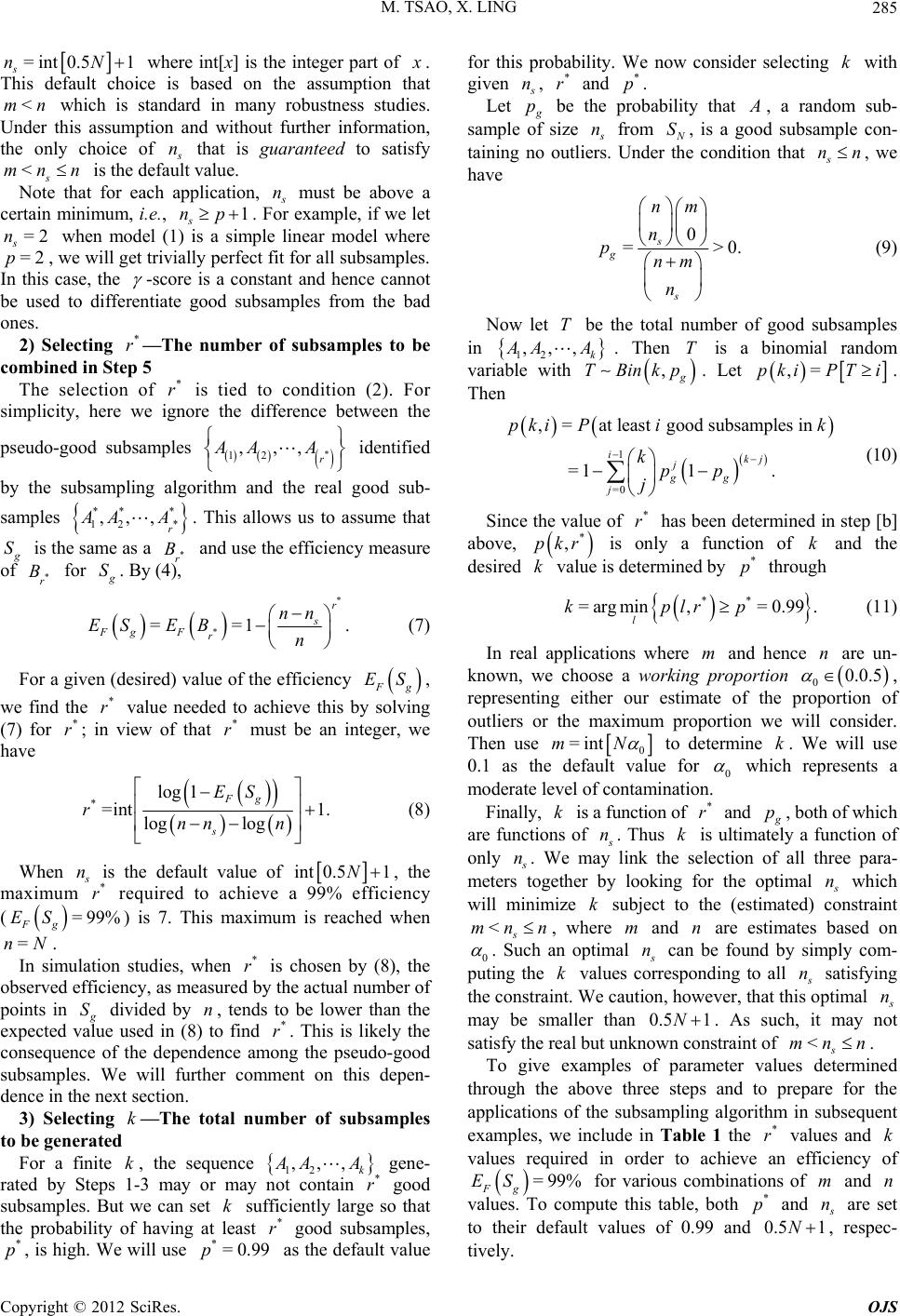 M. TSAO, X. LING 285 = sint0.51nN where int[x] is the integer part of . This default choice is based on the assumption that which is standard in many robustness studies. Under this assumption and without further information, the only choice of <mn n that is guaranteed to satisfy is the default value. <mn s Note that for each application, n n 1np =2 must be above a certain minimum, i.e., s. For example, if we let when model (1) is a simple linear model where , we will get trivially perfect fit for all subsamples. In this case, the s n =2p -score is a constant and hence cannot be used to differentiate good subsamples from the bad ones. 2) Selecting —The number of subsamples to be combined in Step 5 * r * r * 12 ,, ** * 12 * ,,, r The selection of is tied to condition (2). For simplicity, here we ignore the difference between the pseudo-good subsamples identified AA , r A by the subsampling algorithm and the real good sub- samples AA. This allows us to assume that S B is the same as a * r and use the efficiency measure of for B * r S. By (4), * 1 . r s nn n * == Fg Fr ES EB (7) For a given (desired) value of the efficiency g ES * r * r , we find the value needed to achieve this by solving (7) for ; in view of that must be an integer, we have * r *log 1 =int log s rnn 1. log Fg ES n (8) When n is the default value of int 0.51N , the maximum required to achieve a 99% efficiency * r 99% Fg ES * r () is 7. This maximum is reached when = =nN . In simulation studies, when is chosen by (8), the observed efficiency, as measured by the actual number of points in S divided by n, tends to be lower than the expected value used in (8) to find . This is likely the consequence of the dependence among the pseudo-good subsamples. We will further comment on this depen- dence in the next section. * r k k,,, 3) Selecting —The total number of subsamples to be generated For a finite , the sequence 12 k AA * r k gene- rated by Steps 1-3 may or may not contain good subsamples. But we can set sufficiently large so that the probability of having at least good subsamples, , is high. We will use as the default value for this probability. We now consider selecting with given k r *=0.99p * * p n* r* p, and . Let p be the probability that , a random sub- sample of size n from S s nn , is a good subsample con- taining no outliers. Under the condition that , we have 0 =>0. s g s nm n pnm n T (9) Now let be the total number of good subsamples in ,,, k12 AA. Then T is a binomial random variable with , TBinkp . Let ,=pkiPT i. Then 1 =0 ,=at least good subsamples in =11 . ikj j gg j pki Pik kpp j * r (10) Since the value of has been determined in step [b] above, * ,pkr k* p is only a function of k and the desired value is determined by through ** =argmin ,=0.99 l kplrp m n . (11) In real applications where and hence are un- known, we choose a working proportion 0.0.5 0, representing either our estimate of the proportion of outliers or the maximum proportion we will consider. Then use 0 =intmN to determine . We will use 0.1 as the default value for k 0 which represents a moderate level of contamination. Finally, is a function of and k* r p, both of which are functions of n k. Thus is ultimately a function of only n. We may link the selection of all three para- meters together by looking for the optimal n which will minimize subject to the (estimated) constraint k <s mn n , where and are estimates based on 0 m n . Such an optimal n k can be found by simply com- puting the values corresponding to all n satisfying the constraint. We caution, however, that this optimal n 0.5 1N <s mn n may be smaller than . As such, it may not satisfy the real but unknown constraint of . To give examples of parameter values determined through the above three steps and to prepare for the applications of the subsampling algorithm in subsequent examples, we include in Table 1 the values and values required in order to achieve an efficiency of * rk = 99%ES m n * p Fg for various combinations of and values. To compute this table, both and n 0.5 1N are set to their default values of 0.99 and , respec- ively. t Copyright © 2012 SciRes. OJS 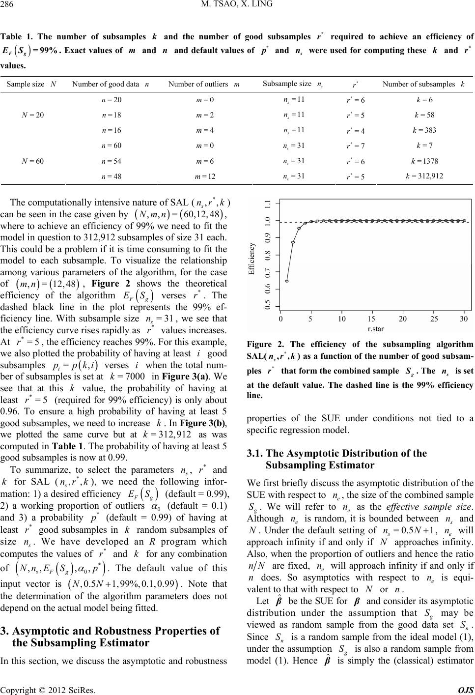 M. TSAO, X. LING OJS 286 k* r Table 1. The number of subsamples and the number of good subsamples required to achieve an efficiency of = 99% Fg ES m n. Exact values of and and default values of * and were used for computing these and values. s nk* r Nn m Sample size Number of good data Number of outliers Subsample size n* rk Number of subsamples =20n=0mn* r=6k =11 s =6 =18 n=2mn* r=5 8 k =2N =16 n=4mn* r=3 83 k =60 n=0mn* r=7k =54 n=6mnr=1378 k=6N =48 n=12mn=312,912 k =11 s =5 0 =11 s =4 =31 s =7 =31 s *=6 0 =31 s *=5r The computationally intensive nature of SAL () can be seen in the case given by * ,, s nrk , ,Nmn =60,12, 48 ,=12,mn , where to achieve an efficiency of 99% we need to fit the model in question to 312,912 subsamples of size 31 each. This could be a problem if it is time consuming to fit the model to each subsample. To visualize the relationship among various parameters of the algorithm, for the case of , Figure 2 shows the theoretical efficiency of the algorithm 48 g verses . The dashed black line in the plot represents the 99% ef- ficiency line. With subsample size , we see that the efficiency curve rises rapidly as values increases. At , the efficiency reaches 99%. For this example, we also plotted the probability of having at least good subsamples i verses when the total num- ber of subsamples is set at in Figure 3(a). We see that at this value, the probability of having at least (required for 99% efficiency) is only about 0.96. To ensure a high probability of having at least 5 good subsamples, we need to increase . In Figure 3(b), we plotted the same curve but at as was computed in Table 1. The probability of having at least 5 good subsamples is now at 0.99. ES =31 s n * r i 00 k = 312k * r =5 i ,912 * r r =,ki =70k pp k *=5 Figure 2. The efficiency of the subsampling algorithm SAL( ) as a function of the number of good subsam- ples that form the combined sample * ,, s nrk * r . The is set at the default value. The dashed line is the 99% efficiency line. s n n properties of the SUE under conditions not tied to a specific regression model. 3.1. The Asymptotic Distribution of the Subsampling Estimator To summarize, to select the parameters n* r k* ,,nrk , and for SAL (s), we need the following infor- mation: 1) a desired efficiency g ES (default = 0.99), 2) a working proportion of outliers 0 (default = 0.1) and 3) a probability (default = 0.99) of having at least good subsamples in random subsamples of size * p * r k n Nn . We have developed an R program which computes the values of and for any combination * r * 0 , , gp k We first briefly discuss the asymptotic distribution of the SUE with respect to e, the size of the combined sample Sn n . We will refer to e as the effective sample size. Although e is random, it is bounded between Copyright © 2012 SciRes. of . The default value of this ,0.5 1,99%,0.1,0.99NN n N=0.51 s nNn N and . Under the default setting of , e will approach infinity if and only if approaches infinity. Also, when the proportion of outliers and hence the ratio ,, sF E SnN n ne Nn ˆ are fixed, e will approach infinity if and only if does. So asymptotics with respect to n is equi- valent to that with respect to or . input vector is . Note that the determination of the algorithm parameters does not depend on the actual model being fitted. be the SUE for Let and consider its asymptotic distribution under the assumption that S S S may be viewed as random sample from the good data set n. Since n is a random sample from the ideal model (1), under the assumption 3. Asymptotic and Robustness Properties of the Subsampling Estimator S ˆ is also a random sample from model (1). Hence is simply the (classical) estimator In this section, we discuss the asymptotic and robustness 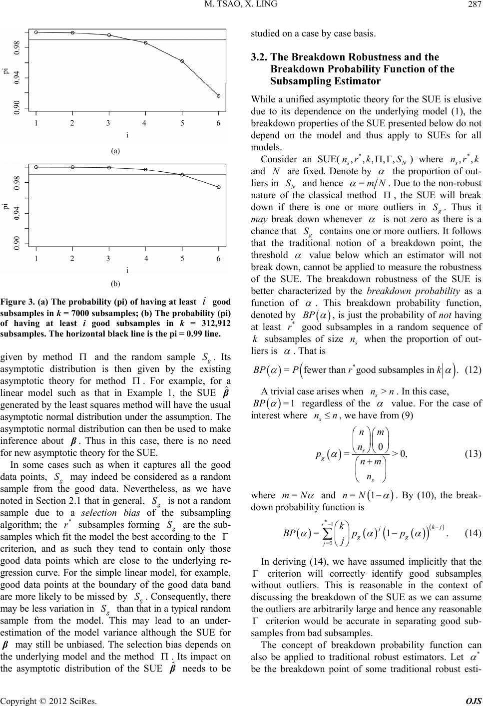 M. TSAO, X. LING 287 (a) (b) Figure 3. (a) The probability (pi) of having at least good subsamples in k = 7000 subsamples; (b) The probability (pi) of having at least i good subsamples in k = 312,912 subsamples. The horizontal black line is the pi = 0.99 line. i given by method and the random sample S ˆ . Its asymptotic distribution is then given by the existing asymptotic theory for method . For example, for a linear model such as that in Example 1, the SUE generated by the least squares method will have the usual asymptotic normal distribution under the assumption. The asymptotic normal distribution can then be used to make inference about . Thus in this case, there is no need for new asymptotic theory for the SUE. In some cases such as when it captures all the good data points, S may indeed be considered as a random sample from the good data. Nevertheless, as we have noted in Section 2.1 that in general, S * r is not a random sample due to a selection bias of the subsampling algorithm; the subsamples forming S are the sub- samples which fit the model the best according to the criterion, and as such they tend to contain only those good data points which are close to the underlying re- gression curve. For the simple linear model, for example, good data points at the boundary of the good data band are more likely to be missed by S. Consequently, there may be less variation in S than that in a typical random sample from the model. This may lead to an under- estimation of the model variance although the SUE for may still be unbiased. The selection bias depends on the underlying model and the method . Its impact on the asymptotic distribution of the SUE ˆ needs to be studied on a case by case basis. 3.2. The Breakdown Robustness and the Breakdown Probability Function of the Subsampling Estimator While a unified asymptotic theory for the SUE is elusive due to its dependence on the underlying model (1), the breakdown properties of the SUE presented below do not depend on the model and thus apply to SUEs for all models. Consider an SUE(* ,,,,, N) where s and are fixed. Denote by nrk S * ,,nrk N the proportion of out- liers in S and hence =mN . Due to the non-robust nature of the classical method , the SUE will break down if there is one or more outliers in S. Thus it may break down whenever is not zero as there is a chance that S contains one or more outliers. It follows that the traditional notion of a breakdown point, the threshold value below which an estimator will not break down, cannot be applied to measure the robustness of the SUE. The breakdown robustness of the SUE is better characterized by the breakdown probability as a function of . This breakdown probability function, denoted by BP , is just the probability of not having at least good subsamples in a random sequence of subsamples of size * r k n when the proportion of out- liers is . That is * =fewer than good subsamples in BPPrk . > s nn (12) A trivial case arises when . In this case, =1BP regardless of the value. For the case of interest where s nn , we have from (9) 0 =>0, s g s nm n pnm n =mN (13) =1nNwhere and *1 =0 =1 rkj j gg j k BPp p j . By (10), the break- down probability function is . (14) In deriving (14), we have assumed implicitly that the criterion will correctly identify good subsamples without outliers. This is reasonable in the context of discussing the breakdown of the SUE as we can assume the outliers are arbitrarily large and hence any reasonable criterion would be accurate in separating good sub- samples from bad subsamples. The concept of breakdown probability function can also be applied to traditional robust estimators. Let * be the breakdown point of some traditional robust esti- Copyright © 2012 SciRes. OJS 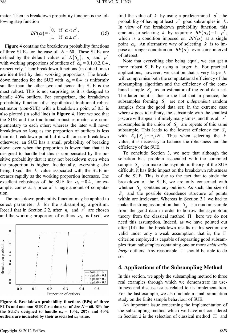 M. TSAO, X. LING 288 mator. Then its breakdown probability function is the fol- lowing step function 0, =1, BP * * if , if . =60N (15) Figure 4 contains the breakdown probability functions of three SUEs for the case of . These SUEs are defined by the default values of ES , n* p = 0.1,0.2,0.4 and with working proportions of outliers of 0 , respectively. Their breakdown functions (in dotted lines) are identified by their working proportions. The break- down function for the SUE with 0=0.4 is uniformly smaller than the other two and hence this SUE is the most robust. This is not surprising as it is designed to handle 40% outliers. For comparison, the breakdown probability function of a hypothetical traditional robust estimator (non-SUE) with a breakdown point of 0.3 is also plotted (in solid line) in Figure 4. Here we see that the SUE and the traditional robust estimator are com- plementary to each other; whereas the later will never breakdown so long as the proportion of outliers is less than its breakdown point but it will for sure breakdown otherwise, an SUE has a small probability of breaking down even when the proportion is lower than that it is designed to handle but this is compensated by the po- sitive probability that it may not breakdown even when the proportion is higher. Incidentally, everything else being fixed, the value associated with the SUE in- creases rapidly as the working proportion increases. The excellent robustness of the SUE for 0 k =0.4 , for ex- ample, comes at a price of a huge amount of computa- tion. The breakdown probability function may be applied to select parameter for the subsampling algorithm. Recall that in Section 2.2, after k n* r 0 and are chosen and the working proportion of outliers is fixed, we Figure 4. Breakdown probability functions (BPs) of three SUEs and one non-SUE for a data set of size N = 60. BPs for the SUE’s designed to handle α0 = 10%, 20% and 40% outliers are indicated by their associated α0 value. find the value of by using a predetermined , the probability of having at least good subsamples in . In view of the breakdown probability function, this amounts to selecting by requiring 0 k* p * rk k * =1BP p , which is a condition imposed on BP at a single point 0 . An alternative way of selecting is to im- pose a stronger condition on k BP over some interval of interest. Note that everything else being equal, we can get a more robust SUE by using a larger k. For practical applications, however, we caution that a very large will compromise both the computational efficiency of the subsampling algorithm and the efficiency of the com- bined sample k S as an estimator of the good data set. The latter point is due to the fact that in practice, the subsamples forming S * r are not independent random samples from the good data set; in the extreme case where k goes to infinity, the subsample with the smallest γ-score will appear infinitely many times, and thus all subsamples in the union of S are repeats of this same subsample. This leads to the lowest efficiency for S with =ESnNk Fgs . Thus when selecting the value, it is necessary to balance the robustness and the efficiency of the SUE. To conclude Section 3, we note that although the selection bias problem associated with the combined sample S can make the asymptotic theory of the SUE difficult, it has little impact on the breakdown robustness of the SUE. This is due to the fact that to study the breakdown of the SUE, we are only concerned with whether S contains any outliers. As such, the size of S and the possible dependence structure of points within are irrelevant. Whereas in Section 3.1 we had to make the strong assumption that S is a random sample from the good data in order to borrow the asymptotic theory from the classical method , here we do not need this assumption. Indeed, as we have pointed out after (14) that the breakdown results in this section are valid under only a weak assumption, that is, the criterion employed is capable of separating good subsam- ples from subsamples containing one or more arbitrarily large outliers. Any reasonable should be able to do so. 4. Applications of the Subsampling Method In this section, we apply the subsampling method to three real examples through which we demonstrate its use- fulness and discuss issues related to its implementation. For the last example, we also include a small simulation study on the finite sample behaviour of SUE. An important issue concerning the implementation of the subsampling method which we have not considered in Section 2 is the selection of classical method and Copyright © 2012 SciRes. OJS 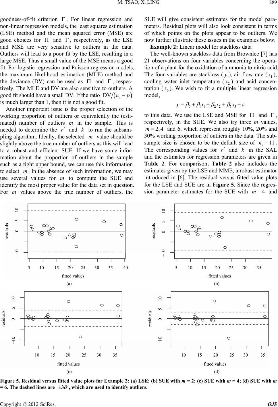 M. TSAO, X. LING OJS 289 Copt © SciR yrigh 2012es. goodness-of-fit criterion . For linear regression and non-linear regression models, the least squares estimation (LSE) method and the mean squared error (MSE) are good choices for and , respectively, as the LSE and MSE are very sensitive to outliers in the data. Outliers will lead to a poor fit by the LSE, resulting in a large MSE. Thus a small value of the MSE means a good fit. For logistic regression and Poisson regression models, the maximum likelihood estimation (MLE) method and the deviance (DV) can be used as and , respec- tively. The MLE and DV are also sensitive to outliers. A good fit should have a small DV. If the ratio DV e np is much larger than 1, then it is not a good fit. Another important issue is the proper selection of the working proportion of outliers or equivalently the (esti- mated) number of outliers in the sample. This is needed to determine the and to run the subsam- pling algorithm. Ideally, the selected value should be slightly above the true number of outliers as this will lead to a robust and efficient SUE. If we have some infor- mation about the proportion of outliers in the sample such as a tight upper bound, we can use this information to select . In the absence of such information, we may use several values for to compute the SUE and identify the most proper value for the data set in question. For values above the true number of outliers, the SUE will give consistent estimates for the model para- meters. Residual plots will also look consistent in terms of which points on the plots appear to be outliers. We now further illustrate these issues in the examples below. Example 2: Linear model for stackloss data m k m * r m y The well-known stackloss data from Brownlee [7] has 21 observations on four variables concerning the opera- tion of a plant for the oxidation of ammonia to nitric acid. The four variables are stackloss (), air flow rate (1 ), cooling water inlet temperature (2 ) and acid concen- tration (3 ). We wish to fit a multiple linear regression model, 0112233 =yxxx m m to this data. We use the LSE and MSE for and , respectively, in the SUE. We also try three m values, and 6, which represent roughly 10%, 20% and 30% working proportion of outliers in the data. The sub- sample size is chosen to be the default size of s. The corresponding values for and k in the SAL and the estimates for regression parameters are given in Table 2. For comparison, Table 2 also includes the estimates given by the LSE and MME, a robust estimator introduced in [6]. The residual versus fitted value plots for the LSE and SUE are in Figure 5. Since the regres- sion parameter estimates for the SUE with and =2 ,4m =11n * r =4m (a) (b) (c) (d) Figure 5. Residual versus fitted value plots for Example 2: (a) LSE; (b) SUE with m = 2; (c) SUE with m = 4; (d) SUE with m = 6. The dashed lines are ˆ 3, which are used to identify outliers. 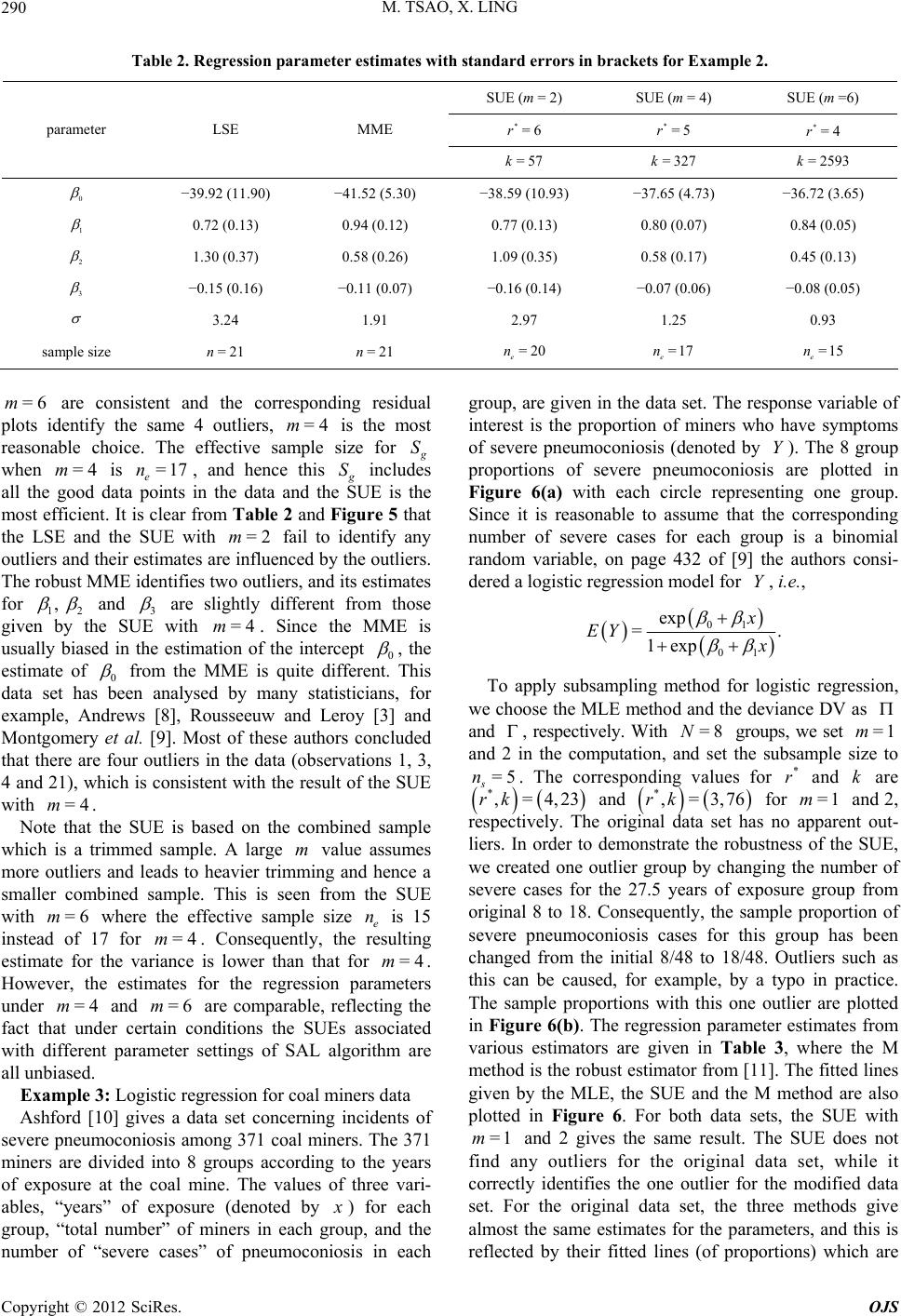 M. TSAO, X. LING 290 Table 2. Regression parameter estimates with standard errors in brackets for Example 2. SUE (m = 2) SUE (m = 4) SUE (m =6) *=6r*=5r*=4r parameter LSE MME =5k=3k=2593k7 27 0 −39.92 (11.90) −41.52 (5.30) −38.59 (10.93) −37.65 (4.73) −36.72 (3.65) 0.72 (0.13) 0.94 (0.12) 0.77 (0.13) 0.80 (0.07) 0.84 (0.05) 1 2 1.30 (0.37) 0.58 (0.26) 1.09 (0.35) 0.58 (0.17) 0.45 (0.13) 3 −0.15 (0.16) −0.11 (0.07) −0.16 (0.14) −0.07 (0.06) −0.08 (0.05) 3.24 1.91 2.97 1.25 0.93 sample size =2 n=2n=2 e n=1 e n=15 e n 1 1 0 7 =6m =4 are consistent and the corresponding residual plots identify the same 4 outliers, m is the most reasonable choice. The effective sample size for S =4m=1n when is e, and hence this 7 S =2 includes all the good data points in the data and the SUE is the most efficient. It is clear from Table 2 and Figure 5 that the LSE and the SUE with fail to identify any outliers and their estimates are influenced by the outliers. The robust MME identifies two outliers, and its estimates for 12 m , and 3 are slightly different from those given by the SUE wi=4. Since the MME is usually biased in the estimation of the intercept 0 th m , the estite of 0 ma from the MME is quite different. This data set has been analysed by many statisticians, for example, Andrews [8], Rousseeuw and Leroy [3] and Montgomery et al. [9]. Most of these authors concluded that there are four outliers in the data (observations 1, 3, 4 and 21), which is consistent with the result of the SUE m with =4. m =6m n m =4m m Note that the SUE is based on the combined sample which is a trimmed sample. A large value assumes more outliers and leads to heavier trimming and hence a smaller combined sample. This is seen from the SUE with where the effective sample size e is 15 instead of 17 for . Consequently, the resulting estimate for the variance is lower than that for . However, the estimates for the regression parameters under and are comparable, reflecting the fact that under certain conditions the SUEs associated with different parameter settings of SAL algorithm are all unbiased. =4 =6=4m Example 3: Logistic regression for coal miners data Ashford [10] gives a data set concerning incidents of severe pneumoconiosis among 371 coal miners. The 371 miners are divided into 8 groups according to the years of exposure at the coal mine. The values of three vari- ables, “years” of exposure (denoted by ) for each group, “total number” of miners in each group, and the number of “severe cases” of pneumoconiosis in each group, are given in the data set. The response variable of interest is the proportion of miners who have symptoms of severe pneumoconiosis (denoted by ). The 8 group proportions of severe pneumoconiosis are plotted in Figure 6(a) with each circle representing one group. Since it is reasonable to assume that the corresponding number of severe cases for each group is a binomial random variable, on page 432 of [9] the authors consi- dered a logistic regression model for , i.e., Y Y 01 01 exp =. 1exp EY To apply subsampling method for logistic regression, we choose the MLE method and the deviance DV as and , respectively. With groups, we set and 2 in the computation, and set the subsample size to . The corresponding values for and k are =8N=1m =5 s n* r *,=4,23rk and *,=3,76rk =1m =1m for and 2, respectively. The original data set has no apparent out- liers. In order to demonstrate the robustness of the SUE, we created one outlier group by changing the number of severe cases for the 27.5 years of exposure group from original 8 to 18. Consequently, the sample proportion of severe pneumoconiosis cases for this group has been changed from the initial 8/48 to 18/48. Outliers such as this can be caused, for example, by a typo in practice. The sample proportions with this one outlier are plotted in Figure 6(b). The regression parameter estimates from various estimators are given in Table 3, where the M method is the robust estimator from [11]. The fitted lines given by the MLE, the SUE and the M method are also plotted in Figure 6. For both data sets, the SUE with and 2 gives the same result. The SUE does not find any outliers for the original data set, while it correctly identifies the one outlier for the modified data set. For the original data set, the three methods give almost the same estimates for the parameters, and this is reflected by their fitted lines (of proportions) which are Copyright © 2012 SciRes. OJS 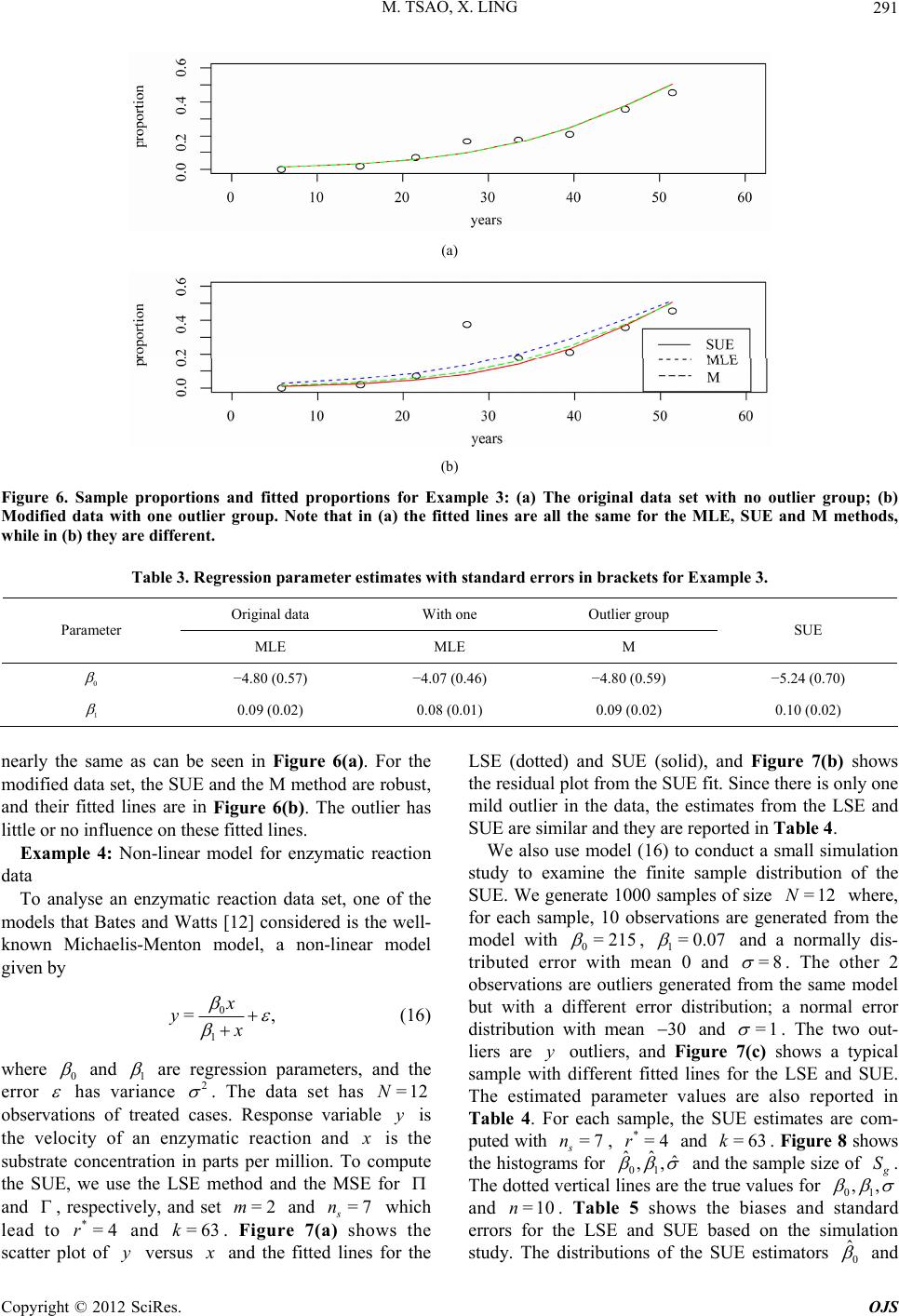 M. TSAO, X. LING 291 (a) (b) Figure 6. Sample proportions and fitted proportions for Example 3: (a) The original data set with no outlier group; (b) Modified data with one outlier group. Note that in (a) the fitted lines are all the same for the MLE, SUE and M methods, while in (b) they are different. Table 3. Regression parameter estimates with standard errors in brackets for Example 3. Original data With one Outlier group Parameter MLE MLE M SUE −4.80 (0.57) −4.07 (0.46) −4.80 (0.59) −5.24 (0.70) 0 1 0.09 (0.02) 0.08 (0.01) 0.09 (0.02) 0.10 (0.02) nearly the same as can be seen in Figure 6(a). For the modified data set, the SUE and the M method are robust, and their fitted lines are in Figure 6(b). The outlier has little or no influence on these fitted lines. Example 4: Non-linear model for enzymatic reaction data To analyse an enzymatic reaction data set, one of the models that Bates and Watts [12] considered is the well- known Michaelis-Menton model, a non-linear model given by 0 1 =, x yx (16) where 0 and 1 are regression parameters, and the error LSE (dotted) and SUE (solid), and Figure 7(b) shows the residual plot from the SUE fit. Since there is only one mild outlier in the data, the estimates from the LSE and SUE are similar and they are reported in Table 4. We also use model (16) to conduct a small simulation study to examine the finite sample distribution of the SUE. We generate 1000 samples of size where, for each sample, 10 observations are generated from the model with 0 =12N =215 , 1=0.07 and a normally dis- tributed error with mean 0 and =8 . The other 2 observations are outliers generated from the same model but with a different error distribution; a normal error distribution with mean 30 and =1 . The two out- liers are outliers, and Figure 7(c) shows a typical sample with different fitted lines for the LSE and SUE. The estimated parameter values are also reported in Table 4. For each sample, the SUE estimates are com- puted with s, and . Figure 8 shows the histograms for 01 y =7n*=4r=63k ˆˆ ˆ ,, 2 has variance . The data set has observations of treated cases. Response variable is the velocity of an enzymatic reaction and =12N y is the substrate concentration in parts per million. To compute the SUE, we use the LSE method and the MSE for and the sample size of S ,, . The dotted vertical lines are the true values for 01 and , respectively, and set and s which lead to and . Figure 7(a) shows the scatter plot of versus =2 =10n 0 ˆ and . Table 5 shows the biases and standard errors for the LSE and SUE based on the simulation study. The distributions of the SUE estimators m=7n =6 *=4r3k y and and the fitted lines for the Copyright © 2012 SciRes. OJS 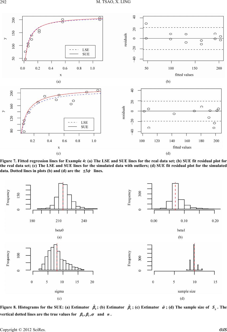 M. TSAO, X. LING 292 (a) (b) (c) (d) Figure 7. Fitted regression lines for Example 4: (a) The LSE and SUE lines for the real data set; (b) SUE fit residual plot for the real data set; (c) The LSE and SUE lines for the simulated data with outliers; (d) SUE fit residual plot for the simulated data. Dotted lines in plots (b) and (d) are the ˆ 3 lines. (a) (b) (c) (d) ˆ0ˆ1ˆ Figure 8. Histograms for the SUE: (a) Estimator ; (b) Estimator ; (c) Estimator ; (d) The sample size of . The vertical dotted lines are the true values for 01 ,, n and . Copyright © 2012 SciRes. OJS 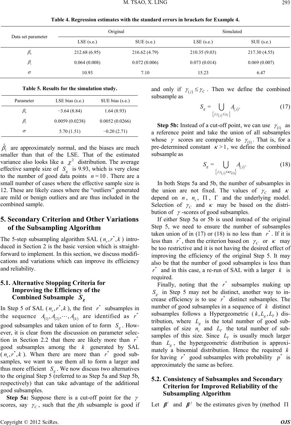 M. TSAO, X. LING 293 Table 4. Regression estimates with the standard errors in brackets for Example 4. Original Simulated Data set parameter LSE (s.e.) SUE (s.e.) LSE (s.e.) SUE (s.e.) 0 212.68 (6.95) 216.62 (4.79) 210.35 (9.03) 217.30 (4.55) 1 0.064 (0.008) 0.072 (0.006) 0.073 (0.014) 0.069 (0.007) 10.93 7.10 15.23 6.47 Table 5. Results for the simulation study. Parameter LSE bias (s.e.) SUE bias (s.e.) 0 −3.64 (8.84) 1.64 (8.93) 1 0.0059 (0.0238) 0.0052 (0.0266) 5.70 (1.51) −0.20 (2.71) 1 ˆ are approximately normal, and the biases are much smaller than that of the LSE. That of the estimated variance also looks like a 2 distribution. The average effective sample size of S =10n * ,,nrk is 9.93, which is very close to the number of good data points . There are a small number of cases where the effective sample size is 12. These are likely cases where the “outliers” generated are mild or benign outliers and are thus included in the combined sample. 5. Secondary Criterion and Other Variations of the Subsampling Algorithm The 5-step subsampling algorithm SAL (s) intro- duced in Section 2 is the basic version which is straight- forward to implement. In this section, we discuss modifi- cations and variations which can improve its efficiency and reliability. 5.1. Alternative Stopping Criteria for Improving the Efficiency of the Combined Subsample In Step 5 of SAL (), the first subsamples in * ,,nrk * r 12 , k s the sequence ,, AA* r are identified as good subsamples and taken union of to form S * r * ,,nrk * . How- ever, it is clear from the discussion on parameter selec- tion in Section 2.2 that there are likely more than good subsamples among the k generated by SAL (s). When there are more than r good sub- samples, we want to use them all to form a larger and thus more efficient S. We now discuss two alternatives to the original Step 5 (referred to as Step 5a and Step 5b, respectively) that can take advantage of the additional good subsamples. Step 5a: Suppose there is a cut-off point for the scores, say C , such that the jth subsample is good if and only if C j . Then we define the combined subsample as : = C j g. j SA (17) Step 5b: Instead of a cut-off point, we can use 1 as a reference point and take the union of all subsamples whose scores are comparable to 1 . That is, for a pre-determined constant >1 , we define the combined subsample as 1 : = j g. j SA (18) In both Steps 5a and 5b, the number of subsamples in the union are not fixed. The values of C and depend on , n n, , and the underlying model. Selection of C and may be based on the distri- bution of -scores of good subsamples. If either Step 5a or 5b is used instead of the original Step 5, we need to ensure the number of subsamples taken union of in (17) or (18) is no less than . If it is less than , then the criterion based on C * r * r or may be too restrictive and it is not having the desired effect of improving the efficiency of the original Step 5. It may also be that the number of good subsamples is less than and in this case, a re-run of SAL with a larger is required. * r k * r Finally, noting that the subsamples making up S * r k ,, in Step 5 may not be distinct, another way to in- crease efficiency is to use distinct subsamples. The number of good subsamples in a sequence of distinct subsamples follows a Hypergeometric ( T) dis- tribution, where kL L L is the total number of good sub- samples of size n L L and T the total number of sub- samples of this size. Since T is usually much larger than L k * r* p i , the hypergeometric distribution is approxi- mately a binomial distribution. Hence the required for having good subsamples with probability is approximately the same as before. 5.2. Consistency of Subsamples and Secondary Criterion for Improved Reliability of the Subsampling Algorithm and be the estimates given by (method Let Copyright © 2012 SciRes. OJS 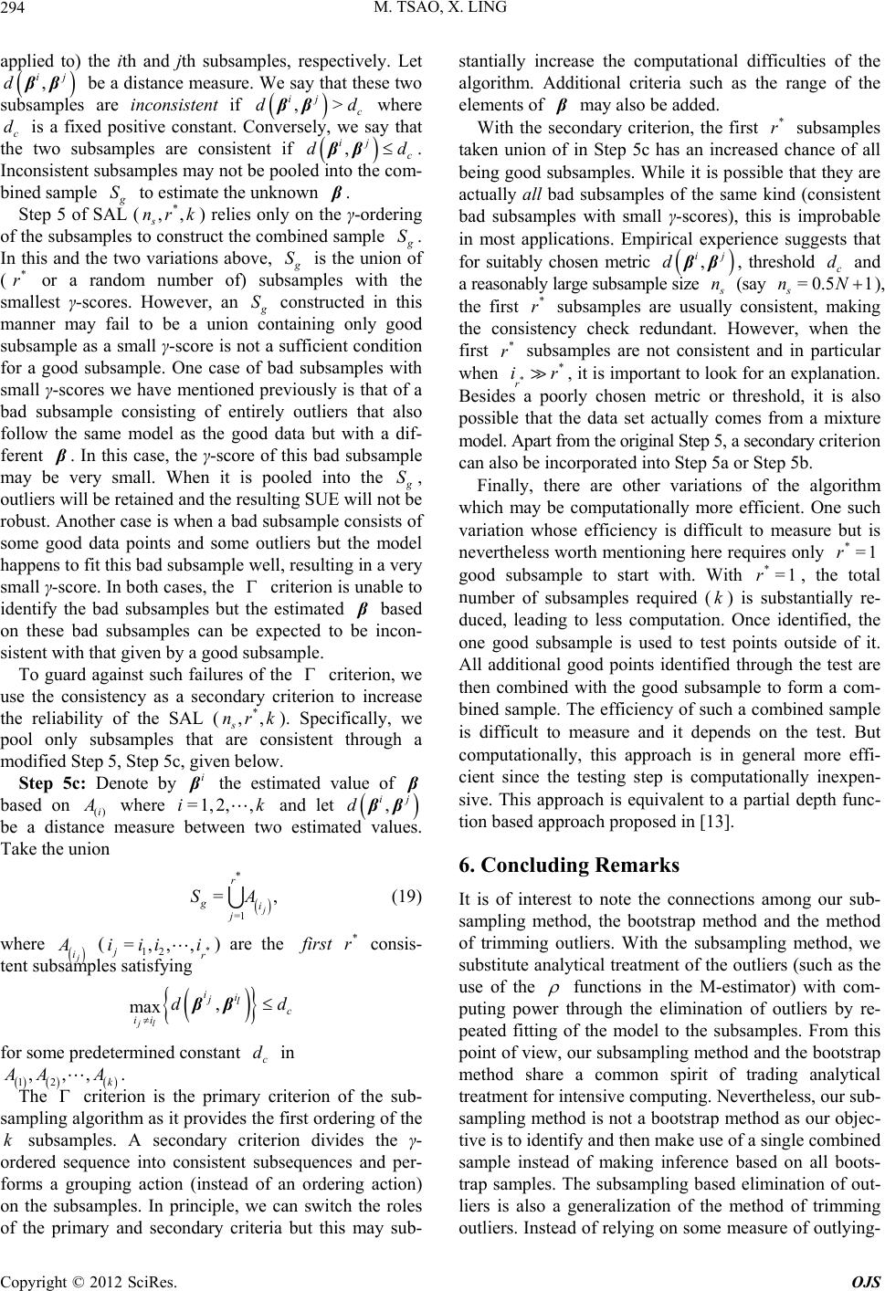 M. TSAO, X. LING 294 applied to) the ith and jth subsamples, respectively. Let , ij dβ be a distance measure. We say that these two subsamples are inconsistent if c where c is a fixed positive constant. Conversely, we say that the two subsamples are consistent if c ,> ij ddββ d , ij dd ββ . Inconsistent subsamples may not be pooled into the com- bined sample S to estimate the unknown . Step 5 of SAL () relies only on the γ-ordering of the subsamples to construct the combined sample * ,, s nrk S. In this and the two variations above, S is the union of ( or a random number of) subsamples with the smallest γ-scores. However, an * r S constructed in this manner may fail to be a union containing only good subsample as a small γ-score is not a sufficient condition for a good subsample. One case of bad subsamples with small γ-scores we have mentioned previously is that of a bad subsample consisting of entirely outliers that also follow the same model as the good data but with a dif- ferent . In this case, the γ-score of this bad subsample may be very small. When it is pooled into the S, outliers will be retained and the resulting SUE will not be robust. Another case is when a bad subsample consists of some good data points and some outliers but the model happens to fit this bad subsample well, resulting in a very small γ-score. In both cases, the criterion is unable to identify the bad subsamples but the estimated based on these bad subsamples can be expected to be incon- sistent with that given by a good subsample. To guard against such failures of the criterion, we use the consistency as a secondary criterion to increase the reliability of the SAL (). Specifically, we pool only subsamples that are consistent through a modified Step 5, Step 5c, given below. k * ,, s nr i Step 5c: Denote by the estimated value of based on ()i where and let =1,2, ,ik , ij dβ be a distance measure between two estimated values. Take the union * =1 = j r gi j S ,A (19) where i (jr ii ) are the first consis- tent subsamples satisfying * 12 =,, ,i i , x jl ii jl iiββ c d * r ,,, ma c dd for some predetermined constant in 12 k AA . The criterion is the primary criterion of the sub- sampling algorithm as it provides the first ordering of the subsamples. A secondary criterion divides the γ- ordered sequence into consistent subsequences and per- forms a grouping action (instead of an ordering action) on the subsamples. In principle, we can switch the roles of the primary and secondary criteria but this may sub- stantially increase the computational difficulties of the algorithm. Additional criteria such as the range of the elements of k may also be added. With the secondary criterion, the first subsamples taken union of in Step 5c has an increased chance of all being good subsamples. While it is possible that they are actually all bad subsamples of the same kind (consistent bad subsamples with small γ-scores), this is improbable in most applications. Empirical experience suggests that for suitably chosen metric * r , ij dβ , threshold and a reasonably large subsample size c d n=0.5 1nN (say s ), the first subsamples are usually consistent, making the consistency check redundant. However, when the first subsamples are not consistent and in particular when * r, it is important to look for an explanation. Besides a poorly chosen metric or threshold, it is also possible that the data set actually comes from a mixture model. Apart from the original Step 5, a secondary criterion can also be incorporated into Step 5a or Step 5b. * r * r * ir *=1r *=1r k Finally, there are other variations of the algorithm which may be computationally more efficient. One such variation whose efficiency is difficult to measure but is nevertheless worth mentioning here requires only good subsample to start with. With , the total number of subsamples required () is substantially re- duced, leading to less computation. Once identified, the one good subsample is used to test points outside of it. All additional good points identified through the test are then combined with the good subsample to form a com- bined sample. The efficiency of such a combined sample is difficult to measure and it depends on the test. But computationally, this approach is in general more effi- cient since the testing step is computationally inexpen- sive. This approach is equivalent to a partial depth func- tion based approach proposed in [13]. 6. Concluding Remarks It is of interest to note the connections among our sub- sampling method, the bootstrap method and the method of trimming outliers. With the subsampling method, we substitute analytical treatment of the outliers (such as the use of the functions in the M-estimator) with com- puting power through the elimination of outliers by re- peated fitting of the model to the subsamples. From this point of view, our subsampling method and the bootstrap method share a common spirit of trading analytical treatment for intensive computing. Nevertheless, our sub- sampling method is not a bootstrap method as our objec- tive is to identify and then make use of a single combined sample instead of making inference based on all boots- trap samples. The subsampling based elimination of out- liers is also a generalization of the method of trimming outliers. Instead of relying on some measure of outlying- Copyright © 2012 SciRes. OJS  M. TSAO, X. LING Copyright © 2012 SciRes. OJS 295 REFERENCES ness of the data to decide which data points to trim, the subsampling method uses a model based trimming by identifying subsamples containing outliers through fitting the model to the subsamples. The outliers are in this case outliers with respect to the underlying regression model instead of some measure of central location and they are only implicitly identified as being part of the data points not in the final combined sample. [1] P. J. Huber, “Robust Statistics,” Wiley, New York, 1981. [2] F. R. Hampel, E. M. Ronchetti, P. J. Rousseeuw and W. A. Stahel, “Robust Statistics: The Approach Based on In- fluence Functions,” Wiley, New York, 1986. [3] P. J. Rousseeuw and A. M. Leroy, “Robust Regression and Outlier Detection,” Wiley, New York, 1987. [4] R. A. Maronna, R. D. Martin and V. J. Yohai, “Robust Statistics: Theory and Methods,” Wiley, New York, 2006. The subsampling method has two main advantages: it is easy to use and it can be used for any regression model to produce robust estimation for the underlying ideal model. There are, however, important theoretical issues that remain to be investigated. These include the charac- terization of the dependence structure among observa- tions in the combined sample, the finite sample distri- bution and the asymptotic distribution of the SUE. Un- fortunately, there does not seem to be a unified approach which can be used to tackle these issues for SUEs for all regression models; the dependence structure and the distributions of the SUE will depend on the underlying regression model as well as the method and criterion chosen. This is yet another similarity to the bootstrap method in that although the basic ideas of such com- putation intensive methods have wide applications, there is no unified theory covering all applications and one needs to investigate the validity of the methods on a case by case basis. We have made some progress on the sim- ple case of a linear model. We continue to examine these issues for this and other models, and hope to report our findings once they become available. [5] D. G. Simpson, D. Ruppert and R. J. Carroll, “On One- Step GM-Estimates and Stability of Inferences in Linear Regression,” Journal of the American Statistical Associa- tion, Vol. 87, No. 418, 1992, pp. 439-450. [6] V. J. Yohai, “High Breakdown-Point and High Efficiency Estimates for Regression,” Annals of Statistics, Vol. 15, No. 2, 1987, pp. 642-656. doi:10.1214/aos/1176350366 [7] K. A. Brownlee, “Statistical Theory and Methodology in Science and Engineering,” 2nd Edition, Wiley, New York, 1965. [8] D. F. Andrews, “A Robust Method for Multiple Linear Regression,” Technometrics, Vol. 16, No. 4, 1974, pp. 523-531. [9] D. C. Montgomery, E. A. Peck and G. G. Vining, “Intro- duction to Linear Regression Analysis,” 4th Edition, Wiley, New York, 2006. [10] J. R. Ashford, “An Approach to the Analysis of Data for Semi-Quantal Responses in Biological Assay,” Biomet- rics, Vol. 15, No. 4, 1959, pp. 573-581. doi:10.2307/2527655 [11] E. Cantoni and E. Ronchetti, “Robust Inference for Gen- eralized Linear Models,” Journal of American Statistical Association, Vol. 96, No. 455, 2001, pp. 1022-1030. doi:10.1198/016214501753209004 7. Acknowledgements [12] D. M. Bates and D. G. Watts, “Nonlinear Regression Analysis and Its Applications,” Wiley, New York, 1988. The authors would like to thank Dr. Julie Zhou for her generous help and support throughout the development of this work. This work was supported by a grant from the National Science and Engineering Research Council of Canada. [13] M. Tsao, “Partial Depth Functions for Multivariate Data,” Manuscript in Preparation, 2012.  M. TSAO, X. LING 296 Appendix: Proofs of Theorems 1 and 2 Proof of Theorem 1: Let p be the probability that random subsample of size n from S >0p ** ,,AA l ,,AA >0 * is a good subsample containing no outliers. Since , we have . s g With probability 1, the subsequence 12 is an infinite sequence. This is so because the event that this subsequence contains only finitely many subsamples is equivalent to the event that there exists a finite such that 1ll contains no good subsamples. Since g, the probability of this latter event and hence that of the former event are both zero. Further, under the condition that nn p n S, * may be viewed as a ran- dom sample of size n ** ,,AA taken directly without replace- ment from n. Hence with probability 1, 12 is an infinite sequence of random samples from the finite population n. It follows that for any S S n zS , the probability that it is in at least one of the * i is 1. Hence n. This and the fact that imply the theorem. PS B n BS * =BA =1 Proof of Theorem 2: We prove (4) by induction. For , since 11 which contains exactly =1j n points, is a constant and 1 W 1 ==. 1 F EB EW n nn =1j E Hence (4) is true for . To find 2F, denote by B* 1 the complement of * 1 with respect to n. Then S* 1 contains nn points. Since 2 * is a random sample of size n S taken without replacement from n, we may assume it contains 1 data points from U* 1 and 1s nU data points from * 1 . It follows that has a hypergeo- metric distribution 1 U ,,, ss nnnn 1HypergU (20) with expected value 1 EU =. s s nn nn ** 21 =BAA 1 .U 21 2 == =1 . sss s nn EWnEUn nn nn nn Since 2 , its number of data points Hence 2 = s Wn It follows that 2 2=1, s F nn EB n =2j 12j j # and formula (4) is also true for . Now assume (4) holds for some . We show that it also holds for . Denote by the number of points in . Then * =# =#= 11 1 jjjjj WB BAWU , where 1 U is the number of good data points in B1 but not in B . The distribution of U1 conditioning on 11 = j Ww is 11 11 =Hyperg,,, jj jjs UW wnnwn 1j (21) By (21) and the assumption that (4) holds for , we have 111 1 1 1 1 1 = = = =1 ==1. jj jj j js s sj j s ss jj ss j EWEWEEUW nW EWE nn nn nEW n nn nnn n nn nn nn n n It follows that ==1 . js Fj EW nn EB nn j Thus (4) also holds for , which proves Theorem 2. Copyright © 2012 SciRes. OJS
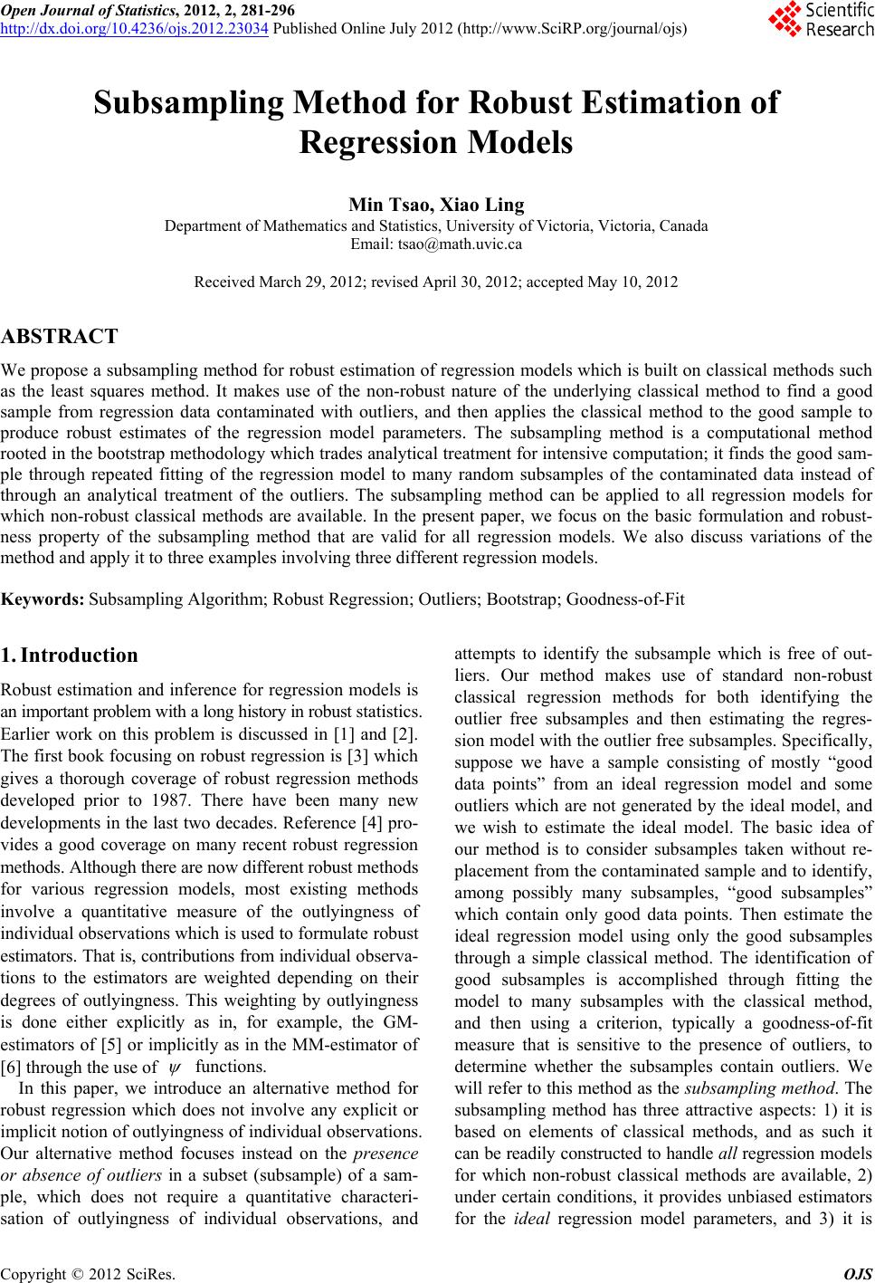
|