Open Journal of Statistics, 2012, 2, 309-312
http://dx.doi.org/10.4236/ojs.2012.23038 Published Online July 2012 (http://www.SciRP.org/journal/ojs)
A Revision of AIC for Normal Error Models
Kunio Takezawa
Agroinformatics Division, Agricultural Research Center, National Agriculture and Food Research Organization,
Graduate School of Life and Environmental Sciences, University of Tsukuba, Tsukuba, Japan
Email: nonpara@gmail.com
Received March 21, 2012; revised April 22, 2012; accepted May 4, 2012
ABSTRACT
Conventional Akaike’s Information Criterion (AIC) for normal error models uses the maximum-likelihood estimator of
error variance. Other estimators of error variance, however, can be employed for defining AIC for normal error models.
The maximization of the log-likelihood using an adjustable error variance in light of future data yields a revised version
of AIC for normal error models. It also gives a new estimator of error variance, which will be called the “third variance”.
If the model is described as a constant plus normal error, which is equivalent to fitting a normal distribution to
one-dimensional data, the approximated value of the third variance is obtained by replacing (n 1) (n is the number of
data) of the unbiased estimator of error variance with (n 4). The existence of the third variance is confirmed by a sim-
ple numerical simulation.
Keywords: AIC; AICc; Normal Error Models; Third Variance
1. Introduction
Akaike’s Information Criterion (AIC) for multiple linear
models with normal i.i.d. errors is defined as (e.g., [1,2])



2
log 2πlog2 4q
ˆˆ
2,, 24,
j
AICnnRSS nn
la q

 Xy
2
11
ˆˆ ,
ji
j i
ij
a xy





1
i
(1)
where n is the number of data and q is the number of
predictors of the multiple linear model. Hence, the num-
ber of regression coefficients in this model is (q + 1)
when the error variance is regarded as a regression coef-
ficient. X is a design matrix composed of the predictor
values in the data. y is the vector composed of values of
the target variable in the data. RSS stands for the residual
sum of squares:
0
q
n
RSS a
 (2)
where are the estimators of regression
coefficients of a multiple linear model. xij(1 i n, 1 j
q) is an element of X.
01
ˆˆ ˆ
,, ,
q
aa a
y
in

is an element of y.

2
ˆˆ
,,
j
la
Xy

is the log-likeli- hood of the regression
model in light of the data at hand. It is defined as



22
ˆˆ ˆ
,, log2πlog .
222
j
nnn
la

 Xy

ˆˆ
,,aa
2
ˆ
(3)
The multiple linear model for obtaining Equations (1)
and (3) contains 01 given by the least squares
method (also called the maximum likelihood method for
normal errors), and the error variance (
ˆ
,
q
a
) given by the
maximum likelihood method. 2
ˆ
is derived using
2
ˆ.RSS n
(4)
2
ˆ
defined above is used as the error variance in AIC
because AIC is a statistic based on the maximum-likeli-
hood estimator. However, the unbiased error variance
shown below rather than the maximum-likelihood esti-
mator of error variance is utilized in most statistical cal-
culations.

2
ˆ1
ub RSS n q
. (5)
The maximum-likelihood estimator of error variance may
not be the only choice for the error variance for AIC.
Hence, in this paper, we discusses the adjustment of error
variance to calculate AIC for normal error models after
recalling the derivation of conventional AIC for normal
error models. Then, this consideration leads to a new
estimator of error variance, which will be called the
“third variance”. Finally, the existence of the third vari-
ance is shown by a simple numerical simulation.
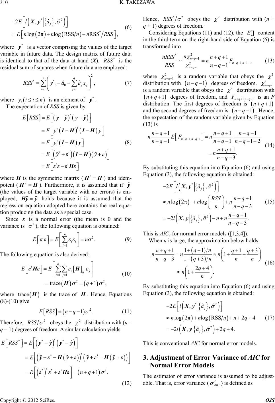
2. Derivation of AIC for Normal Error
Models
Conventional AIC for normal error models is easily de-
rived when the multiple linear model with normal error
assumed by an analyst contains the real equation pro-
ducing the data as a special case. AIC based on these
assumption is an approximation of
C
opyright © 2012 SciRes. OJS
K. TAKEZAWA
310


 
*2
ˆˆ
2, ,
log 2πlog RSS
j
El a
Enn n




Xy
*
RSS ,
n RSS
*
y
*
RSS
2
11
ˆˆ
,
q
ijij
ij
a x





(6)
where is a vector comprising the values of the target
variable in future data. The design matrix of future data
is identical to that of the data at hand (X). is the
residual sum of squares when future data are employed:
**
0
n
RSSy a
(7)
where i
y
iin *
y


ˆ
Ey







y
IHy
y
IH ε
t
is an element of .
The expectation of RSS is given by





ˆt
t
t
t
tt
tt
ERSS E
E
E
E







yy y
yIH
yIH
yε
εε εHε
(8)
where H is the symmetric matrix (
H
2
) and idem-
potent (
H
H
y

). Furthermore, it is assumed that if
(the values of the target variable with no errors) is em-
ployed,
H
yy
ε
2
holds because it is assumed that the
regression equation adopted here contains the real equa-
tion producing the data as a special case.
Since is a normal error (the mean is 0 and the
variance is
), the following equation is obtained:
2
1
.
ii n
n
t
i
EE





 
22
1 ,
ij
ij
q



εε (9)
The following equation is also derived:

11
trace
nn
t
ij
EE


H




εHε
H

trace
(10)
where
H
is the trace of
H
. Hence, Equations
(8)-(10) give

2
1n q.ERSS
 (11)
Therefore, 2
RSS
obeys the 2
distribution with (n
q – 1) degrees of freedom. A similar calculation yields





***
**
**
ˆˆ
t
t
tt
ERSS E
E
En






 





yyyy
yεHy εyε
εεεHε


2
1.
q

Hy ε
(12)
Hence, *2
RSS 2
obeys the
distribution with (n +
q + 1) degrees of freedom.
Considering Equations (11) and (12), the content
in the third term on the right-hand side of Equation (6) is
transformed into
[]E
2
*
1
1,1 1
2
1
1
~.
1
nq
nq n
nq
n
nRSSn q
nF
RSSn q

 



2
(13)
2
where 1nq
is a random variable that obeys the
distribution with
1nq
2
degrees of freedom. 1nq
is a random variable that obeys the 2
distribution with
1nq
1
F
degrees of freedom, and 1,nq nq  is an F
distribution. The first degrees of freedom is
1nq

1nq
and the second degrees of freedom is . Hence,
the expectation of the random variable given by Equation
(13) is
1, 1
111
1112
1.
3
nq nq
nqnq nq
nEF n
nqnq nq
nq
nnq
 







(14)
By substituting this equation into Equation (6) and using
Equation (3), the following equation is obtained:



*2
2
ˆˆ
2, ,
1
log 2π log3
1
ˆˆ
2, ,.
3
j
j
El a
RSSn q
nn n
nnq
nq
la nn
nq






 


 
Xy
Xy
(15)
This is AICc for normal error models ([1,3,4]).
When n is large, the approximation below holds:

11
113
1
31 3
24
1.
qn
nqq q
nn n
nqq nnn
q
nn





 




(16)
By substituting this equation into Equation (6) and using
Equation (3), the following equation is obtained:
 


*2
2
ˆˆ
2, ,
log 2πlog RSS24
ˆˆ
2,, 24.
j
j
El a
nnnnq
la q




 
Xy
Xy
2
AIC
(17)
This is conventional AIC for normal error models.
3. Adjustment of Error Variance of AIC for
Normal Error Models
The estimator of error variance is assumed to be adjust-
able. That is, error variance (
) is defined as
Copyright © 2012 SciRes. OJS
K. TAKEZAWA 311
2
AIC ,RSS n
 (18)
where
is a constant for adjusting error variance. The
use of AIC
2
in
A
c
IC a
c
(Equation (15)) yields
A
IC
(AIC-adjustable):


log 2π
a
c
AIC n
n
log
1.
3
RSS
nn
nq
nq







ˆ
(19)
a
c
A
IC is Then,
which minimizes
324.
1q



2
ˆ
ˆ1
nq
n
nq


 (20)
Hence, the following AIC
is different from the unbi-
ased estimator of error variance:
2
ˆAIC ˆ
RSS n.

2
ˆ
(21)
AIC
will be called the “third variance” because the dis-
covery of this variance follows those of the maximum-
likelihood estimator of error variance and the unbiased
estimator of error variance. In particular, when 0q
which indicates the fitting of a normal distribution to one-
dimensional data. Although 0
or 1
is adopted
conventionally, 4
is preferable in terms of log-like-
lihood in light of future data.
The substitution of Equations (20) and (21) to Equa-
tion (15) leads to



 
log 2π
log 13
3
1
log 2πlog
u
c
AIC n
RSS
nnn nq
nq n
nn nq n
RSS n
nn
nq



 





 
1
1
13
1,
3
nq
q
q
qn









u
(22)
where c
A
IC
u
c
denotes the “ultimate AIC”. Simulation
studies show that the model selection characteristics of
A
IC falls somewhere between
A
IC and c
A
IC

1100yi
.
4. Numerical Simulation
The simulation data consists of (reali-

i
zations of N(13.0, 42)) and
*

1 100yi
0
i
ˆ
a2
ˆ
(realiza-
tions of N(13.0, 42)). ,
, , and are
expressed as follows:
RSS *
RSS

2
0
1
1
ˆˆ
n
i
i
ay
n,,RSSn

2
**
00
11
ˆˆ
,,
nn
ii
y a



(23)

2
ii
RSSy aRSS
(24)
Figure 1. Relationship between
and average
ˆˆ
*2
0
2,
i
lya
. A circle indicates the minimum point of
each line. Ten lines reflect 10 repeats of the simulations.
100n
where
. By altering the seed of random values,
5000 sets of
i
y
and
*
i
y are obtained. Then, 5000
*2
0
ˆˆ
2,
i
lya
values of are obtained and averaged.
This procedure is carried out using one of the values
9.8, 9.6, 9.4,,10 as
.
Figure 1 shows the result of this simulation. Ten lines
show that the simulation is repeated 10 times by chang-
ing the seed of random values. Each minimum point is
located around the
4
point; these ten points appar-
ently deviate from the
1
and
0
4
points. This
shows that
gives a better log-likelihood in light
of future data and that the third variance should be con-
sidered.
5. Conclusion
A
The error variance for IC
u
is adjustable. The optimiza-
tion of the errror variance yields c
A
IC in which the
third variance is adopted as the error variance. The third
variance is different from both the unbiased estimator of
error variance and the maximum-likelihood estimator of
error variance. The features and usage of the third vari-
ance remains to be elucidated.
REFERENCES
[1] K. P. Burnham and D. R. Anderson, “Model Selection
and Multi-Model Inference A Practical Information-
Theoretic Approach,” Springer, Berlin, 2010.
[2] S. Konishi and G. Kitagawa, “Information Criteria and
Statistical Modeling,” Springer, Berlin, 2007.
[3] C. M. Hurvich and C.-L. Tsai, “Regression and Time
Series Model Selection in Small Samples,” Biometrika,
Vol. 76, No. 2, 1989, pp. 297-307.
doi:10.1093/biomet/76.2.297
Copyright © 2012 SciRes. OJS
K. TAKEZAWA
Copyright © 2012 SciRes. OJS
312
[4] N. Sugiura, “Further Analysis of the Data by Akaike’s
Information Criterion and Finite Corrections,” Commu-
nications in Statistics-Theory and Methods, Vol. 7, No. 1,
1978, pp. 13-26. doi:10.1080/03610927808827599