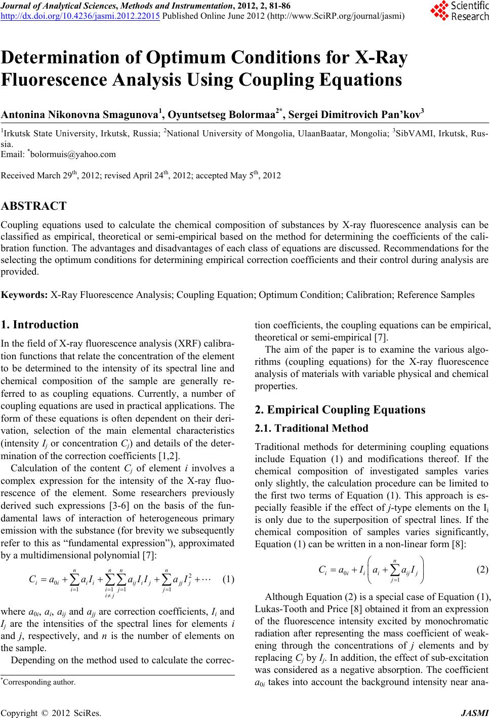
Journal of Analytical Sciences, Methods and Instrumentation, 2012, 2, 81-86
http://dx.doi.org/10.4236/jasmi.2012.22015 Published Online June 2012 (http://www.SciRP.org/journal/jasmi)
81
Determination of Optimum Conditions for X-Ray
Fluorescence Analysis Using Coupling Equations
Antonina Nikonovna Smagunova1, Oyuntsetseg Bolormaa2*, Sergei Dimitrovich Pan’kov3
1Irkutsk State University, Irkutsk, Russia; 2National University of Mongolia, UlaanBaatar, Mongolia; 3SibVAMI, Irkutsk, Rus-
sia.
Received March 29th, 2012; revised April 24th, 2012; accepted May 5th, 2012
ABSTRACT
Coupling equations used to calculate the chemical composition of substances by X-ray fluorescence analysis can be
classified as empirical, theoretical or semi-empirical based on the method for determining the coefficients of the cali-
bration function. The advantages and disadvantages of each class of equations are discussed. Recommendations for the
selecting the optimum conditions for determining empirical correction coefficients and their control during analysis are
provided.
Keywords: X-Ray Fluorescence Analysis; Coupling Equation; Optimum Condition; Calibration; Reference Samples
1. Introduction
In the field of X-ray fluorescence analysis (XRF) calibra-
tion functions that relate the concentration of the element
to be determined to the intensity of its spectral line and
chemical composition of the sample are generally re-
ferred to as coupling equations. Currently, a number of
coupling equations are used in practical applications. The
form of these equations is often dependent on their deri-
vation, selection of the main elemental characteristics
(intensity Ij or concentration Cj) and details of the deter-
mination of the correction coefficients [1,2].
Calculation of the content Cj of element i involves a
complex expression for the intensity of the X-ray fluo-
rescence of the element. Some researchers previously
derived such expressions [3-6] on the basis of the fun-
damental laws of interaction of heterogeneous primary
emission with the substance (for brevity we subsequently
refer to this as “fundamental expression”), approximated
by a multidimensional polynomial [7]:
2
0
111 1
nnn n
ii iiijijjjj
iij j
ij
CaaIaII aI
 

 
  (1)
where а0i, ai, aij and ajj are correction coefficients, Ii and
Ij are the intensities of the spectral lines for elements i
and j, respectively, and n is the number of elements on
the sample.
Depending on the method used to calculate the correc-
tion coefficients, the coupling equations can be empirical,
theoretical or semi-empirical [7].
The aim of the paper is to examine the various algo-
rithms (coupling equations) for the X-ray fluorescence
analysis of materials with variable physical and chemical
properties.
2. Empirical Coupling Equations
2.1. Traditional Method
Traditional methods for determining coupling equations
include Equation (1) and modifications thereof. If the
chemical composition of investigated samples varies
only slightly, the calculation procedure can be limited to
the first two terms of Equation (1). This approach is es-
pecially feasible if the effect of j-type elements on the Ii
is only due to the superposition of spectral lines. If the
chemical composition of samples varies significantly,
Equation (1) can be written in a non-linear form [8]:
0
1
n
iiii ijj
j
Ca IaaI


 



(2)
Although Equation (2) is a special case of Equation (1),
Lukas-Tooth and Price [8] obtained it from an expression
of the fluorescence intensity excited by monochromatic
radiation after representing the mass coefficient of weak-
ening through the concentrations of j elements and by
replacing Cj by Ij. In addition, the effect of sub-excitation
was considered as a negative absorption. The coefficient
а0i takes into account the background intensity near ana-
*Corresponding author.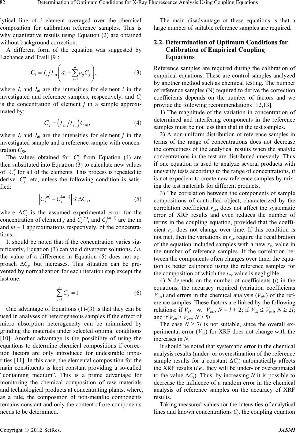

Determination of Optimum Conditions for X-Ray Fluorescence Analysis Using Coupling Equations
82
lytical line of i element averaged over the chemical
composition for calibration reference samples. This is
why quantitative results using Equation (2) are obtained
without background correction.
A different form of the equation was suggested by
Lachance and Traill [9]:
0
1
,
n
iiij
ii
j
aCCIIa





j

(3)
where Ii and Ii0 are the intensities for element i in the
investigated and reference samples, respectively, and Cj
is the concentration of element j in a sample approxi-
mated by:

00
,
j
jx jj
I
ICC (4)
where I
j and Ij0 are the intensities for element j in the
investigated sample and a reference sample with concen-
tration Cj0.
The values obtained for
j
C

from Equation (4) are
then substituted into Equation (3) to calculate new values
of
j
C for all of the elements. This process is repeated to
derive
j
C etc, unless the following condition is satis-
fied:
 
1, mm
j
j
CC C


j
(5)
where ΔCj is the assumed experimental error for the
concentration of element j and Сj
(m), and Cj (m–1) are the m
and m – 1 approximations respectively, of the concentra-
tions.
It should be noted that if the concentration varies sig-
nificantly, Equation (3) can yield divergent solutions, i.e.
the value of a difference in Equation (5) does not ap-
proach ΔCj, but increases. This situation can be pre-
vented by normalization for each iteration step except the
last one:
1
1
n
j
j
C


 (6)
One advantage of Equations (1)-(3) is that they can be
used in analyses of heterogeneous samples if the effect of
micro absorption heterogeneity can be minimized by
grinding the materials under selected optimal conditions
[10]. Another advantage is the possibility of using the
equations to determine chemical compositions if correc-
tion factors are only introduced for undesirable impu-
rities [11]. In this case, the elemental composition for the
main constituents is kept constant providing a so-called
“containing medium”. This is a prime advantage for
monitoring the chemical composition of raw materials
and technological products at concentrating plants, where,
as a rule, the composition of non-metallic components
remains constant and only the content of ore components
needs to be determined.
The main disadvantage of these equations is that a
large number of suitable reference samples are required.
2.2. Determination of Optimum Conditions for
Calibration of Empirical Coupling
Equations
Reference samples are required during the calibration of
empirical equations. These are control samples analyzed
by another method such as chemical testing. The number
of reference samples (N) required to derive the correction
coefficients depends on the number of factors and we
provide the following recommendations [12,13].
1) The magnitude of the variation in concentration of
determined and interfering components in the reference
samples must be not less than that in the test samples.
2) A non-uniform distribution of reference samples in
terms of the range of concentrations does not decrease
the correctness of the analytical results when the analyte
concentrations in the test are distributed unevenly. Thus
if one equation is used to analyze several products with
unevenly tests according to the range of concentrations, it
is not expedient to create new reference samples by mix-
ing the test materials for different products.
3) The correlation between the components of sample
compositions of controlled object, characterized by the
correlation coefficient rxy, does not affect the systematic
error of XRF results and even reduces the number of
terms in the coupling equation, provided that the coeffi-
cient rxy does not change over time. If this condition is
not met, then the variations in rxy require the recalibration
of the equation included samples with a new rxy value in
the number of reference samples. If the correlation be-
tween the components often changes over time, the equa-
tion is better calibrated using the reference samples for
the composition of which the rxy value is negligible.
4) N depends on the number of coefficients (l) in the
equations, the accuracy required (variation coefficients
Vext) and errors in the chemical analysis (Vch.) of the ref-
erence samples. These factors are linked by the following
relations: if Vch. Vext, N = l + 2; if Vch  Vext, N  2l;
and if Vch > Vext, N > 5l.

The case N  7l is not suitable, since the overall ex-
perimental error (Vch) for XRF does not change with the
increases in N.
It should be noted that systematic error in the chemical
analysis results (under- or overestimation of the reference
sample results for a constant ΔCj) automatically affects
the XRF results (i.e., they will be under- or overestimated
to the value ΔCj). Thus, by increasing N it is possible to
decrease the influence of a random error in the chemical
analysis of reference samples on the accuracy of XRF
results.
Taking measured values for the intensities of analytical
lines and known concentrations Cj, the coupling equation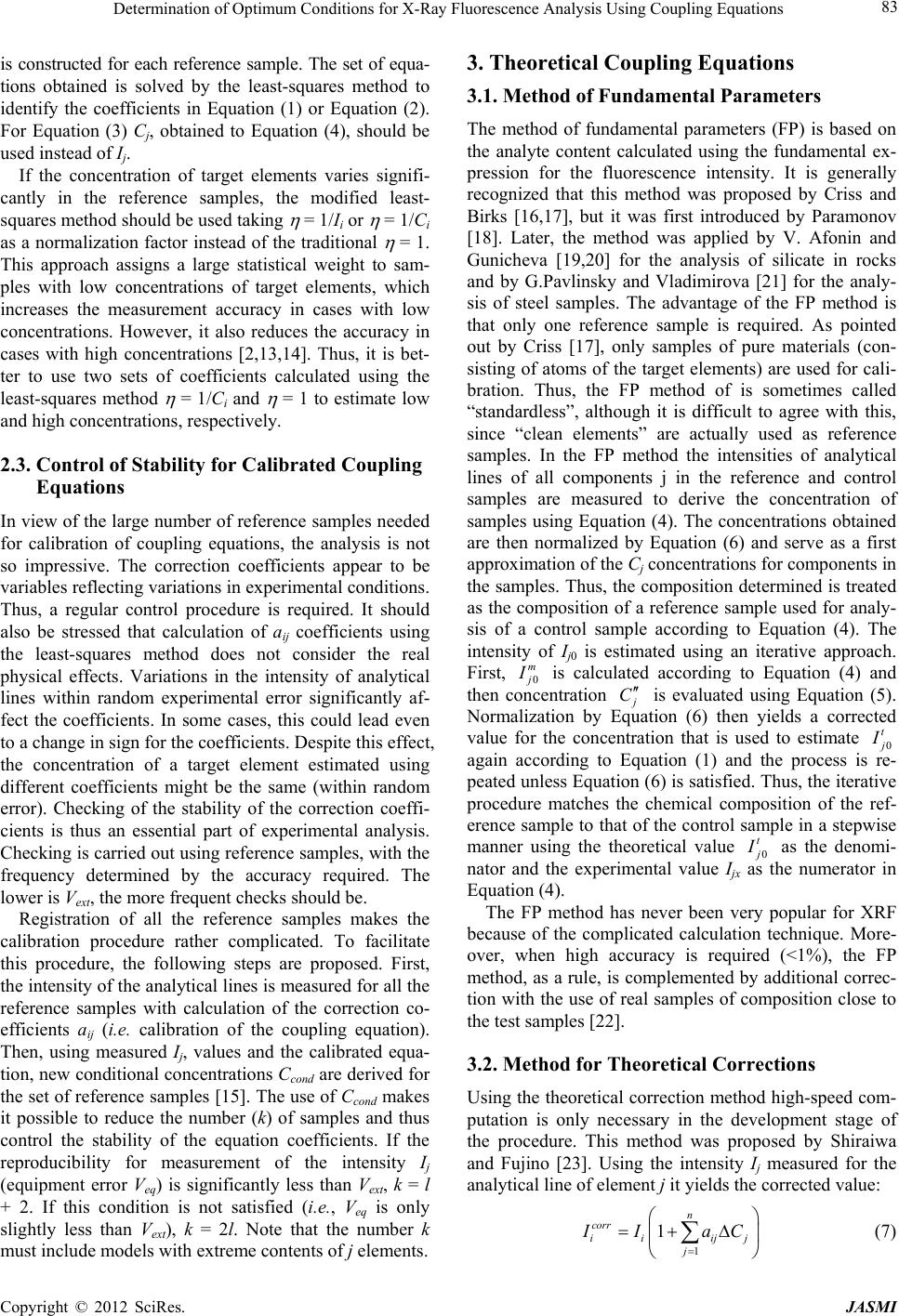

Determination of Optimum Conditions for X-Ray Fluorescence Analysis Using Coupling Equations 83
is constructed for each reference sample. The set of equa-
tions obtained is solved by the least-squares method to
identify the coefficients in Equation (1) or Equation (2).
For Equation (3) Cj, obtained to Equation (4), should be
used instead of Ij.
If the concentration of target elements varies signifi-
cantly in the reference samples, the modified least-
squares method should be used taking
 = 1/Ii or  = 1/Ci
as a normalization factor instead of the traditional  = 1.
This approach assigns a large statistical weight to sam-
ples with low concentrations of target elements, which
increases the measurement accuracy in cases with low
concentrations. However, it also reduces the accuracy in
cases with high concentrations [2,13,14]. Thus, it is bet-
ter to use two sets of coefficients calculated using the
least-squares method
 = 1/Ci and  = 1 to estimate low
and high concentrations, respectively.
2.3. Control of Stability for Calibrated Coupling
Equations
In view of the large number of reference samples needed
for calibration of coupling equations, the analysis is not
so impressive. The correction coefficients appear to be
variables reflecting variations in experimental conditions.
Thus, a regular control procedure is required. It should
also be stressed that calculation of aij coefficients using
the least-squares method does not consider the real
physical effects. Variations in the intensity of analytical
lines within random experimental error significantly af-
fect the coefficients. In some cases, this could lead even
to a change in sign for the coefficients. Despite this effect,
the concentration of a target element estimated using
different coefficients might be the same (within random
error). Checking of the stability of the correction coeffi-
cients is thus an essential part of experimental analysis.
Checking is carried out using reference samples, with the
frequency determined by the accuracy required. The
lower is Vext, the more frequent checks should be.
Registration of all the reference samples makes the
calibration procedure rather complicated. To facilitate
this procedure, the following steps are proposed. First,
the intensity of the analytical lines is measured for all the
reference samples with calculation of the correction co-
efficients aij (i.e. calibration of the coupling equation).
Then, using measured Ij, values and the calibrated equa-
tion, new conditional concentrations Сcond are derived for
the set of reference samples [15]. The use of Сcond makes
it possible to reduce the number (k) of samples and thus
control the stability of the equation coefficients. If the
reproducibility for measurement of the intensity Ij
(equipment error Veq) is significantly less than Vext, k = l
+ 2. If this condition is not satisfied (i.e., Veq is only
slightly less than Vext), k = 2l. Note that the number k
must include models with extreme contents of j elements.
3. Theoretical Coupling Equations
3.1. Method of Fundamental Parameters
The method of fundamental parameters (FP) is based on
the analyte content calculated using the fundamental ex-
pression for the fluorescence intensity. It is generally
recognized that this method was proposed by Criss and
Birks [16,17], but it was first introduced by Paramonov
[18]. Later, the method was applied by V. Afonin and
Gunicheva [19,20] for the analysis of silicate in rocks
and by G.Pavlinsky and Vladimirova [21] for the analy-
sis of steel samples. The advantage of the FP method is
that only one reference sample is required. As pointed
out by Criss [17], only samples of pure materials (con-
sisting of atoms of the target elements) are used for cali-
bration. Thus, the FP method of is sometimes called
“standardless”, although it is difficult to agree with this,
since “clean elements” are actually used as reference
samples. In the FP method the intensities of analytical
lines of all components j in the reference and control
samples are measured to derive the concentration of
samples using Equation (4). The concentrations obtained
are then normalized by Equation (6) and serve as a first
approximation of the Cj concentrations for components in
the samples. Thus, the composition determined is treated
as the composition of a reference sample used for analy-
sis of a control sample according to Equation (4). The
intensity of Ij0 is estimated using an iterative approach.
First, 0
т
j
I
is calculated according to Equation (4) and
then concentration
j
C

 is evaluated using Equation (5).
Normalization by Equation (6) then yields a corrected
value for the concentration that is used to estimate 0
t
j
I
again according to Equation (1) and the process is re-
peated unless Equation (6) is satisfied. Thus, the iterative
procedure matches the chemical composition of the ref-
erence sample to that of the control sample in a stepwise
manner using the theoretical value 0
t
j
I
as the denomi-
nator and the experimental value Ijх as the numerator in
Equation (4).
The FP method has never been very popular for XRF
because of the complicated calculation technique. More-
over, when high accuracy is required (<1%), the FP
method, as a rule, is complemented by additional correc-
tion with the use of real samples of composition close to
the test samples [22].
3.2. Method for Theoretical Corrections
Using the theoretical correction method high-speed com-
putation is only necessary in the development stage of
the procedure. This method was proposed by Shiraiwa
and Fujino [23]. Using the intensity Ij measured for the
analytical line of element j it yields the corrected value:
1
1
n
corr
ii ij
j
j
I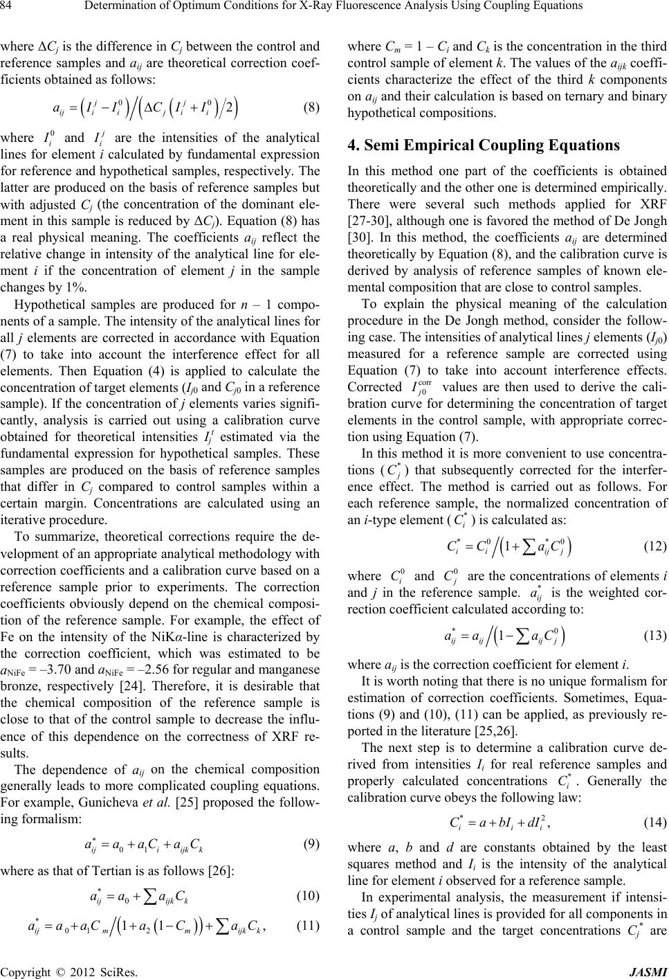
IaC


 



(7)

Determination of Optimum Conditions for X-Ray Fluorescence Analysis Using Coupling Equations
84
where ΔCj is the difference in Cj between the control and
reference samples and aij are theoretical correction coef-
ficients obtained as follows:


 
02 jj
ijiij ii
aII CII 
0
(8)
where 0
i
I
and
j
i
I
are the intensities of the analytical
lines for element i calculated by fundamental expression
for reference and hypothetical samples, respectively. The
latter are produced on the basis of reference samples but
with adjusted Cj (the concentration of the dominant ele-
ment in this sample is reduced by ΔCj). Equation (8) has
a real physical meaning. The coefficients aij reflect the
relative change in intensity of the analytical line for ele-
ment i if the concentration of element j in the sample
changes by 1%.
Hypothetical samples are produced for n – 1 compo-
nents of a sample. The intensity of the analytical lines for
all j elements are corrected in accordance with Equation
(7) to take into account the interference effect for all
elements. Then Equation (4) is applied to calculate the
concentration of target elements (Ij0 and Cj0 in a reference
sample). If the concentration of j elements varies signifi-
cantly, analysis is carried out using a calibration curve
obtained for theoretical intensities Ij
t estimated via the
fundamental expression for hypothetical samples. These
samples are produced on the basis of reference samples
that differ in Сj compared to control samples within a
certain margin. Concentrations are calculated using an
iterative procedure.
To summarize, theoretical corrections require the de-
velopment of an appropriate analytical methodology with
correction coefficients and a calibration curve based on a
reference sample prior to experiments. The correction
coefficients obviously depend on the chemical composi-
tion of the reference sample. For example, the effect of
Fe on the intensity of the NiKα-line is characterized by
the correction coefficient, which was estimated to be
aNiFe = –3.70 and aNiFe = –2.56 for regular and manganese
bronze, respectively [24]. Therefore, it is desirable that
the chemical composition of the reference sample is
close to that of the control sample to decrease the influ-
ence of this dependence on the correctness of XRF re-
sults.
The dependence of aij on the chemical composition
generally leads to more complicated coupling equations.
For example, Gunicheva et al. [25] proposed the follow-
ing formalism:
01ijiijk k
aaaCaC
  (9)
where as that of Tertian is as follows [26]:
*
0ijijk k
aa aC
 (10)
 
*
01 2
11
ijmmijk k
aaaCa CaC 

where Cm = 1 – Ci and Ck is the concentration in the third
control sample of element k. The values of the aijk coeffi-
cients characterize the effect of the third k components
on aij and their calculation is based on ternary and binary
hypothetical compositions.
4. Semi Empirical Coupling Equations
In this method one part of the coefficients is obtained
theoretically and the other one is determined empirically.
There were several such methods applied for XRF
[27-30], although one is favored the method of De Jongh
[30]. In this method, the coefficients aij are determined
theoretically by Equation (8), and the calibration curve is
derived by analysis of reference samples of known ele-
mental composition that are close to control samples.
To explain the physical meaning of the calculation
procedure in the De Jongh method, consider the follow-
ing case. The intensities of analytical lines j elements (Ij0)
measured for a reference sample are corrected using
Equation (7) to take into account interference effects.
Corrected corr
0
j
I values are then used to derive the cali-
bration curve for determining the concentration of target
elements in the control sample, with appropriate correc-
tion using Equation (7).
In this method it is more convenient to use concentra-
tions (*
j
C) that subsequently corrected for the interfer-
ence effect. The method is carried out as follows. For
each reference sample, the normalized concentration of
an i-type element () is calculated as:
*
i
C


*0 *0
1
ii ijj
CC aC
 (12)
where and
0
i
C0
j
C are the concentrations of elements i
and j in the reference sample. is the weighted cor-
rection coefficient calculated according to:
*
ij
a


*
1
ijijij j
aa aC
0
2
i
(13)
where aij is the correction coefficient for element i.
It is worth noting that there is no unique formalism for
estimation of correction coefficients. Sometimes, Equa-
tions (9) and (10), (11) can be applied, as previously re-
ported in the literature [25,26].
The next step is to determine a calibration curve de-
rived from intensities Ii for real reference samples and
properly calculated concentrations . Generally the
calibration curve obeys the following law:
*
i
C
*,
ii
Ca bIdI  (14)
where a, b and d are constants obtained by the least
squares method and Ii is the intensity of the analytical
line for element i observed for a reference sample.
In experimental analysis, the measurement if intensi-
ties Ij of analytical lines is provided for all components in
a control sample and the target concentrations Cj
* are
, (11)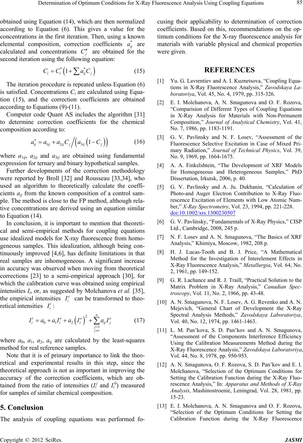

Determination of Optimum Conditions for X-Ray Fluorescence Analysis Using Coupling Equations 85
obtained using Equation (14), which are then normalized
according to Equation (6). This gives a value for the
concentrations in the first iteration. Then, using a known
elemental composition, correction coefficients are
calculated and concentrations
*
ij
a
j
C are obtained for the
second iteration using the following equation:

**
1
ii ijj
CC aC
 

(15)
The iteration procedure is repeated unless Equation (6)
is satisfied. Concentrations Ci are calculated using Equa-
tion (15), and the correction coefficients are obtained
according to Equations (9)-(11).
Computer code Quant AS includes the algorithm [31]
to determine correction coefficients for the chemical
composition according to:



12 3
1
ijijij jijj
aaaCaC
 (16)
where a1ij, a2ij and a3ij are obtained using fundamental
expression for ternary and binary hypothetical samples.
Further developments of the correction methodology
were reported by Broll [32] and Rousseau [33,34], who
used an algorithm to theoretically calculate the coeffi-
cients aij from the known composition of a control sam-
ple. The method is close to the FP method, although rela-
tive concentrations are derived using an equation similar
to Equation (14).
In conclusion, it is important to mention that theoreti-
cal and semi-empirical methods for coupling equations
use idealized models for X-ray fluorescence from homo-
geneous samples. This idealization, although being con-
tinuously improved [4,6], has definite limitations in that
real samples are inhomogeneous. A significant increase
in accuracy was observed when moving from theoretical
corrections [23] to a semi-empirical approach [30], for
which the calibration curve was obtained using empirical
intensities Ii, or, as suggested by Molchanova et al. [35],
the empirical intensities e
i
I
can be transformed to theo-
retical intensities t
i
I
:

2
01 2
1
n
tee
iii
j
ji
e
ijj
I
aaIaI aI


 
 (17)
where a0, a1, a2, aij are calculated by the least-squares
method for real reference samples.
Note that it is of primary importance to link the theo-
retical and experimental results in this step, since the
theoretical approach is not as important in improving the
accuracy of the correction coefficients, which are ob-
tained from the ratio of intensities (Ii
j and Ii 0) measured
for samples of similar chemical composition.
5. Conclusion
The analysis of coupling equations was performed fo-
cusing their applicability to determination of correction
coefficients. Based on this, recommendations on the op-
timum conditions for the X-ray fluorescence analysis for
materials with variable physical and chemical properties
were given.
REFERENCES
[1] Yu. G. Lavrentiev and A. I. Kuznetsova, “Coupling Equa-
tions in X-Ray Fluorescence Analysis,” Zavodskaya La-
boratoriya, Vol. 45, No. 4, 1979, pp. 315-326.
[2] E. I. Molchanova, A. N. Smagunova and O. F. Rozova,
“Comparision of Different Types of Coupling Equations
in X-Ray Analysis for Materials with Non-Permanent
Composition,” Journal of Analytical Chemistry, Vol. 41,
No. 7, 1986, pp. 1183-1191.
[3] G. V. Pavlinsky and N. F. Losev, “Assessment of the
Fluorescence Selective Excitation in Case of Mixed Pri-
mary Radiation,” Journal of Technical Physics, Vol. 39,
No. 9, 1969, pp. 1664-1675.
[4] A. A. Finkelshtein, “The Development of XRF Models
for Homogeneous and Heterogeneous Samples,” PhD
Dissertation, Irkutsk, 2006, p. 40.
[5] G. V. Pavlinsky and A. Ju. Dukhanin, “Calculation of
Photo-and Auger Electron Contribution to X-Ray Fluo-
rescence Excitation of Elements with Low Atomic Num-
ber,” X-Ray Spectrometry, Vol. 23, 1994, pp. 221-228.
doi:10.1002/xrs.1300230507
[6] G. V. Pavlinsky, “Fundamentals of X-Ray Physics,” CISP
Ltd., Cambridge, 2008, 245 p.
[7] N. F. Losev and A. N. Smagunova, “The Basics of XRF
Analysis,” Khimiya, Moscow, 1982, 208 p.
[8] H. J. Lucas-Tooth and B. J. Price, “A Mathematical
Method for the Investigation of Interelement Effects in
X-Ray Fluorescence Analysis,” Metallurgia, Vol. 64, No.
2, 1961, pp. 149-152.
[9] G. R. Lachance and R. J. Traill, “Practical Solution to the
Matrix Problem in X-Ray Analysis,” Canadian Spec-
troscopy, Vol. 11, No. 2, 1966, pр. 43-48.
[10] A. N. Smagunova, N. F. Losev, A. G. Revenko and A. N.
Mejevich, “General Chart of Development the X-Ray
Spectral Analysis Methods,” Zavodskaya Laboratoriya,
Vol. 40, No. 12, 1974, pp. 1461-1463.
[11] L. M. Pan’kova, S. D. Pan’kov and A. N. Smagunova,
“Assessment of the Components Interference Efficiency
Using the Calibration Measurements Method during the
X-Ray Fluorescence Analysis,” Zavodskaya Laboratoriya,
Vol. 44, No. 8, 1978, pp. 950-953.
[12] A. N. Smagunova, O. F. Rozova, S. D. Pan’kov and E. I.
Molchanova, “Selection of the Optimum Conditions for
Setting the Calibration Function during the X-Ray Fluo-
rescence Analysis,” In: Apparatus and Methods of X-Ray
Analysis, Mashinostroenie, Leningrad, Vol. 28, 1981, pp.
15-23.
[13] E. I. Molchanova, A. N. Smagunova and O. F. Rozova,
“Selection of the Optimum Conditions for Setting the
Calibration Function during the X-Ray Fluorescence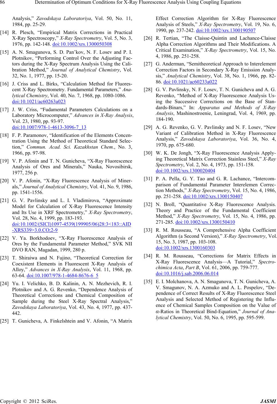

Determination of Optimum Conditions for X-Ray Fluorescence Analysis Using Coupling Equations
86
Analysis,” Zavodskaya Laboratoriya, Vol. 50, No. 11,
1984, pp. 25-29.
[14] R. Plesch, “Empirical Matrix Corrections in Practical
X-Ray Spectroscopy,” X-Ray Spectrometry, Vol. 5, No. 3,
1976, pp. 142-148. doi:10.1002/xrs.1300050308
[15] A. N. Smagunova, S. D. Pan’kov, N. F. Losev and P. I.
Plotnikov, “Performing Control Over the Adjusting Fac-
tors during the X-Ray Spectrum Analysis Using the Cali-
bration Method,” Journal of Analytical Chemistry, Vol.
32, No. 1, 1977, pp. 15-20.
[16] J. Criss and L. Birks, “Calculation Method for Fluores-
cent X-Ray Spectrometry. Fundamental Parameters,” Ana-
lytical Chemistry, Vol. 40, No. 7, 1968, рp. 1080-1086.
doi:10.1021/ac60263a023
[17] J. W. Criss, “Fudamental Parameters Calculations on a
Laboratory Microcomputer,” Advances in X-Ray Analysis,
Vol. 23, 1980, рp. 93-97.
doi:10.1007/978-1-4613-3096-7_13
[18] F. P. Paramonov, “Identification of the Elements Concen-
tration Using the Method of Theoretical Standard Selec-
tion,” Commun. Acad. Sci. Kazakhstan Chem., No. 3,
1966, pp. 97-98.
[19] V. P. Afonin and T. N. Gunicheva, “X-Ray Fluorescence
Analysis of Ores and Minerals,” Nauka, Novosibirsk,
1977, 256 p.
[20] V. P. Afonin, “X-Ray Fluorescence Analysis of Miner-
als,” Journal of Analytical Chemistry, Vol. 41, No. 9, 1986,
pp. 1541-1556.
[21] G. V. Pavlinsky and L. I. Vladimirova, “Approximate
Model for Calculation of X-Ray Fluorescence Intensity
and Its Use in XRF Spectrometry,” X-Ray Spectrometry,
Vol. 28, No. 4, 1999, pp. 183-193.
doi:10.1002/(SICI)1097-4539(199905/06)28:3<183::AID
-XRS339>3.0.CO;2-9
[22] V. Ya. Borkhodoev, “X-Ray Fluorescence Analysis of
Ores by the Fundamental Parameter Method,” SVK NII
DVO RAN, Magadan, 1999, 280 p.
[23] T. Shiraiwa and N. Fujino, “Theoretical Correction for
Coexistent Elements in Fluorescent X-Ray Analysis of
Alloy,” Advances in X-Ray Analysis, Vol. 11, 1968, pp.
63-64. doi:10.1007/978-1-4684-8676-6_5
[24] Yu. I. Velichko, B. D. Kalinin, A. N. Mezhevich, R. I.
Plotnikov and A. G. Revenko, “Dependence Analysis of
Theoretical Corrections and Chemical Composition of
Sample during the Steel X-Ray Spectral Analysis,”
Zavodskaya Laboratoriya, Vol. 43, No. 4, 1977, pp. 437-
442.
[25] T. Gunicheva, A. Finkelshtein and V. Afonin, “A Matrix
Effect Correction Algorithm for X-Ray Fluorescence
Analysis of Steels,” X-Ray Spectrometry, Vol. 19, No. 6,
1990, pр. 237-242. doi:10.1002/xrs.1300190507
[26] R. Tertian, “The Claisse-Quintin and Lachance-Claisse
Alpha Correction Algorithms and Their Modifications. A
Critical Examination,” X-Ray Spectrometry, Vol. 15, No.
4, 1986, рp. 251-258.
[27] G. Anderman, “Semitheoretical Approach to Interelement
Correction Factors in Secondary X-Ray Emission Analy-
sis,” Analytical Chemistry, Vol. 38, No. 1, 1966, pр. 82-
86. doi:10.1021/ac60233a022
[28] G. V. Pavlinsky, N. F. Losev, T. N. Gunicheva and A. G.
Revenko, “Method of X-Ray Fluorescence Analysis Us-
ing the Successive Corrections on the Base of Stan-
dards-Binars,” In: Apparatus and Methods of X-Ray
Analysis, Mashinostroenie, Leningrad, Vol. 4, 1969, pp.
184-190.
[29] A. G. Revenko, G. V. Pavlinsky and N. F. Losev, “New
Variant of Calibration Method in X-Ray Fluorescence
Analysis,” Zavodskaya Laboratoriya, Vol. 36, No. 4,
1970, pp. 675-680.
[30] W. K. De Jongh, “X-Ray Fluorescence Analysis Apply-
ing Theoretical Matrix Correction Stainless Steel,” X-Ray
Spectrometry, Vol. 2, No. 4, 1973, pp. 151-158.
doi:10.1002/xrs.1300020404
[31] P. A. Pella, G. Y. Tao and G. R. Lachance, “Intercom-
parison of Fundamental Parameter Interelemen Correc-
tion Methods,” X-Ray Spectrometry, Vol. 15, No. 4, 1986,
pp. 251-258. doi:10.1002/xrs.1300150407
[32] N. Broll, “Quantitative X-Ray Fluorescence Analysis.
Theory and Practice of the Fundamental Coefficient
Method,” X-Ray Spectrometry, Vol. 15, No. 4, 1986, pр.
271-285. doi:10.1002/xrs.1300150410
[33] R. M. Rousseau, “A Comprehensive Alpha Coefficient
Algorithm (a Second Version),” X-Ray Spectrometry, Vol.
15, No. 3, 1987, pp. 103-108.
doi:10.1002/xrs.1300160303
[34] R. M. Rousseau, “Corrections for Matrix Effects in
X-Ray Fluorescence Analysis—A Tutorial,” Spectro-
chimica Acta, Part B, Vol. 61, 2006, pp. 759-777.
doi:10.1016/j.sab.2006.06.014
[35] E. I. Molchanova, A. N. Smagunova, T. N. Gunicheva, A.
V. Smagunov, N. A. Azmuko and A. L. Pospelov, “De-
pendence of Correct Results of X-Ray Fluorescence Steel
Analysis and Selected Method of Registering the Influ-
ence of Chemical Samples Composition on the Value of
α-Ratios in Theoretical Bind-Equation,” Journal of Ana-
lytical Chemistry, Vol. 50, No. 6, 1995, pp. 595-599.