Journal of Minerals & Materials Characterization & Engineering, Vol. 4, No. 1, pp 11-19, 2005
jmmce.org Printed in the USA. All rights reserved
11
Thermal Properties Of Sediments From Middle Valley
A. Hafaiedh, K. Hassine
Department of Mechanical Engineering,
Institute of High Technology, Nabeul, Tunisia.
Tel: [phone]
Department of Computer Sciences,
University of Sciences, Monastir, Tunisia.
Tel: [phone]
Abstract:
A neural network model was used to treat thermal conductivity data obtained
from Middle Valley. This technique was able to separate the effects of different
parameters such as porosity, grain density, bulk density and water content on the thermal
conductivity. Predicted curves showed good agreement with the experimental results.
Keywords: neural network, thermal conductivity, porosity, grain density, bulk density,
water content.
Introduction
Effective thermal conductivity is an important diffusive transport coefficient to
evaluate the coupled heat and moisture transfer through porous walls so that conduction
heat fluxes may be precisely calculated. This heat transport coefficient in a porous
material may be described in terms of the conductivity of solid matrix and fluid phases
and their quantities, phase change phenomena, and special organization of the phases.
The present work deals with the use of the neural network techniques in order to predict
the dependence of the thermal conductivity as a function of the porosity content for
seafloor massive sulfide deposits.
The marked influence of the different characteristics of the seafloor massive
sulfide bodies and surrounding seafloor materials on the thermal conductivity
measurements opens new directions for field and modeling studies of the combined roles
of conduction and convection in heat transfer at seafloor hydrothermal sites.
There have been extensive experimental and analytical work to investigate the
characteristics and properties of the massive sulfide mounds deposited at major seafloor
hydrothermal sites[1-3] Some of the more interesting work was produced on samples
from the Mid-Atlantic Ridge and the Middle Valley in the Pacific. Rona[2] produced
experimental work on the thermal conductivity of sulfides/sulfates samples from the
volcanic-hosted active sulfide mound in the TAG hydrothermal field in the rift valley of
the mid-Atlantic Ridge, using two different methods. Using the half space divided bar
method, he found that the thermal conductivity of heterogeneous mixtures of sulfide
(predominantly pyrite), quartz, and anhydrite breccias range between 6.1 and 10.4 W/(m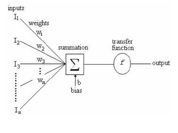

12A. Hafaiedh, K. HassineVol. 4, No. 1
Figure 1: The neuron model
ºK).
Visual and thin-section observations show that many of the Middle Valley
samples used for this study have a matrix rich in clay, silt, and quartz with sulfide veins
irregularly distributed throughout the sediments. These veins as well as the massive
sulfide samples are composed of approximately equal amounts of pyrite and pyrrhotite. It
appears that the matrix composition plays a significant role in the thermal conductivity of
hydrothermal deposits. In particular, the presence or lack of anhydrite within the rock
matrix seems to affect the measurements the most.
The ANN Model
Artificial neural
networks (ANN) are being
used in many different
fields, such as
predictions[4-6], system
designs[7], forecasting and
estimation[8]. They are
composed of simple
computational elements
operating both in parallel
and in sequence, called
neurons or nodes, described
by figure 1. Neurons
process information based
on weighted inputs using
their transfer functions and
sent out outputs. The nodes
in adjacent layers, are fully or partially interconnected with weighted links. The weight
factors play a critical role during the learning process. They start from an initially random
state and move according to the training data sets towards a stable state in a way to
minimize the difference between the actual outputs (target) and the model predicted
outputs. The transfer function of processing nodes is used to determine the output value
of the node based on the total net input from nodes in the prior layer. There are many
different neural net types with each having special properties, so each problem domain
has its own net type. Based on the topology, the connections of an ANN could be either
feedback, where the connections between the nodes form cycles, or feed-forward. The
presence of one or more hidden layers is one of the most important characteristics of
ANN network. The function of neurons in a hidden layer (hidden neurons) is to intervene
between the external input and the network output, in some useful manner, in order to
make the output values converge as close as possible to the target values. The program
keeps adjusting the values of the weights to allow a minimum value of the mean sum
square of the error, then uses the obtained weights in order to calculate the target value.
Using more hidden layers enables the network to extract higher order statistics, in

Vol. 4, No. 1 Thermal Properties Of Sediments From Middle Valley13
particular when the number of the input data is large.
In order to build an ANN model, the number of nodes in both, input and output
layers, the number of hidden layers and the number of nodes in each hidden layer, need to
be defined first. The number of nodes in both input and output layers may be defined
based on the problem to be studied. The number of hidden layers and hidden nodes may
be determined either by the trial and error approach or using some empirical formulas, as
guidance. Kolomogorov's theorem states that twice the number of input variables plus
one is enough hidden nodes to compute any arbitrary continuous function. Carpenter
introduced an equation to define the number of nodes in the hidden layer based on the
number of inputs, and the number of training sample set.
Nh= (Nd / β − No) / (Ni + No)
Where Nh is the number of hidden nodes; Nd is the number of training data pairs; β is the
parameter related to the degree over-determination; Ni is the number of input nodes; and
N is the number of output nodes. In this model, the optimal number of nodes in the
hidden layer is determined by trial and error method.
Experimental Procedure
Measurements were made on vertical and horizontal mini-cores (2.54 cm in
diameter and 2.54 - 3.81 cm in length) from Middle Valley at the Petro-physics
laboratory of the Rosenstiel School of Marine and Atmospheric Sciences in Miami,
Florida. Wet and dry sample weights and volumes were determined using a microbalance
for measuring mass (±0.03%).
Porosity values were determined to approximately ±0.2%, with the assumption
that the porosity is interconnected and the fluid is saturated. The necessary information to
calculate the density porosity and water content was provided by a specifically designed
pycnometer, which employs Archimedes principle of fluid displacement. The displaced
fluid was helium, which assures penetration into crevices and pore spaces in the order of
1 Å (10-10 m). Purge times for 5 min, were made, in order to approach a helium-saturated
steady-state condition. After measuring the wet weights, water was driven off, by keeping
samples at a temperature of 100°C for 24 hr.
Measurements were corrected for salt, assuming a pore-water salinity of 35%, as
required by the American Society for Testing and Materials (ASTM) (D2216, 1989).
Samples were saturated in seawater and placed in a vacuum for 24 hr in order to achieve
situ wet conditions.
The ANN configuration, proposed in this work, has the values of the depth, the
bulk density, the grain density, the pore water volume, and the porosity as inputs and the
corresponding thermal conductivities as outputs. Using this input-output arrangement, we
tried many different network configurations to achieve good performance of the network.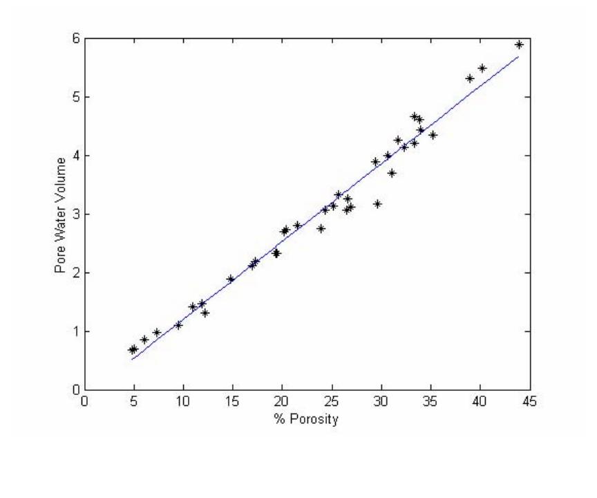

14A. Hafaiedh, K. HassineVol. 4, No. 1
Figure 2: Dependence of the pore water volume on the percent porosity.
The solid lin e was determined by linear fitting
The, five layer, back-propagation model, was considered. It corresponded to the lowest
value of the mean sum square of the error. The first layer is the input layer, with 5
neurons, does not have any computing activity. It was, simply used to enter the values of
the input parameters. The second, third and fourth layers are hidden layers with seven,
five and five neurons, respectively. The fifth layer is the output layer with one neuron,
used to process the outcome for the thermal conductivity. We have chosen the
Levenberg-Marquardt optimization technique[9], which is a powerful algorithm, as a
training algorithm, the log sigmoid function as a transfer function for the first and second
layers and the linear sigmoid function as a transfer function for the output layer.
Results and discussion
Table 1 describes the experimental results obtained for 41 Middle Valley samples.
The pore water volume, PWV, is the ratio of the mass of water in a sediment sample to
the mass of the wet sample. As described by figure 2, PWV shows an almost
proportional dependence on the percent porosity. Equation 1 describes the relationship,
used to calculate the pore water volume for any percent porosity during modeling, which
was determined using a linear fitting program.

Vol. 4, No. 1 Thermal Properties Of Sediments From Middle Valley15
Table 1: Index properties and thermal conductivities of samples from the Middle Valley[1].
#Bulk Density
(g/cm3)
Grain Density
(g/cm3)
Pore Water
Volume (cm3)
% PorosityThermal Conductivity
(W/(mºK))
1 2.862.960.674.822.48
2 2.862.960.704.982.42
3 2.752.860.856.073.91
4 3.854.070.977.314.11
5 2.692.852.028.414.92
6 2.632.801.099.495.10
7 2.662.871.4210.914.67
8 2.773.021.3112.183.98
9 4.324.811.6112.7510.95
10 4.194.751.8914.787.18
11 2.482.832.3319.303.36
12 2.442.792.3319.493.99
13 4.004.753.6019.927.75
14 2.582.992.7220.403.05
15 2.372.802.7423.902.99
16 2.422.883.0624.323.57
17 3.524.363.1425.113.42
18 2.322.813.0726.493.28
19 2.312.793.2626.563.17
20 2.002.743.1126.93.03
21 2.302.853.8829.403.23
22 2.272.813.1729.603.00
23 1.862.693.6931.102.95
24 2.272.894.1332.352.89
25 2.212.814.2033.292.85
26 2.202.804.6633.363.45
27 2.212.844.4333.923.57
28 2.102.815.3138.932.84
29 2.112.875.4940.202.53
30 2.062.895.8943.872.64
PWV = 0.1272P + 0.0509 (1)
Grain density is the ratio of the bulk density minus the porosity to the complement of the
porosity as shown by equation 2. Equation 3 describes the dependence of the bulk
density on both porosity and grain density.
GD = P
PBD
−
−
1(2)
BD = GD (1 – P) + P(3)
Where GD is the grain density, BD is the bulk density, and P is the percent porosity. The
dependences of the thermal conductivity as a function of percent porosity and grain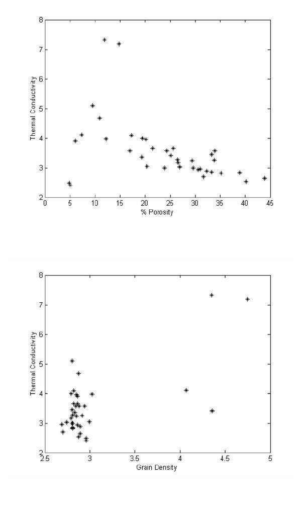

16A. Hafaiedh, K. HassineVol. 4, No. 1
Figure 3a: Dependence of the thermal conductivity on
the porosity (experimental results)
Figure 3b: Dependence of the thermal conductivity on the grain
density fordifferent values of the porosity (experimental results)
density are described in
figures 3a and 3b,
respectively. Results
show no clear
correlations, which may
be due to the fact that
the controlling
parameters of the
thermal dissipation of
heat are changing
simultaneously, making
a separate investigation
of their effects
impossible.
The ANN model
was trained using data in
table 1. The depth, the
bulk density, the grain
density, the pore water
volume, and the porosity
were the dependent
parameters whereas the
thermal conductivity
was the target values.
Results of the ANN
model were then, used
in order to predict the
dependence of the
thermal conductivity on
its influencing
parameters. In all
predictions, the values
of the bulk density were
determined using
equation 3.
Effects of the percent porosity
Figure 4a describes the dependence of the thermal conductivity on the porosity,
for different values of the grain density. In this case, the values of the pore water volume
were determined from the porosity (equation 1). We notice, first a rapid decrease of the
thermal conductivity as a function of the porosity, then decreases slowly. Figure 4b
describes the dependence of the thermal conductivity on the percent porosity for constant
values of the pore water volume. The thermal conductivity decreases rapidly up to a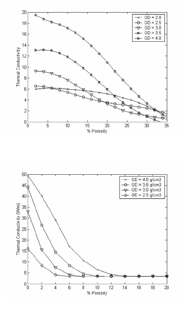

Vol. 4, No. 1 Thermal Properties Of Sediments From Middle Valley17
Figure 4a: Dependence of the thermal conductivity on the porosity for
different values of the grain density. In this case, the value of the pore
water volume is de termined using eq uation 1
Figure 4b: Dependence of the thermal conductivity on the Porosity
for different values of the grain density. In this case,
the value of the pore water volume is constant
somewhat constant
value. Higher grain
density values allowed
higher values of the
thermal conductivity.
Effects of grain density
Figure 5
describes the effects of
the grain density on the
thermal conductivity for
different values of the
porosity. The thermal
conductivity keeps an
almost constant value
then increases rapidly.
This behavior may be
because grains may have
some internal porosity,
which increases as the
grain density decreases.
Conclusions
In this wok, we used the
neural network
technique in order
determine the
dependence of the
thermal conductivity of
Middle Valley samples
on some different
parameters such as
porosity, grain density
and water content. This
technique proved to be
able to separate the
effects of the different
parameters on the thermal conductivity, which is impossible to realize experimentally.
Effects of other parameters such as phase composition, grain size distribution and pore
size distribution could be determined and used in the training procedures for a better
prediction capability.

18A. Hafaiedh, K. HassineVol. 4, No. 1
References
[1] Rona. P.A., Davis, E.E., and Ludwig, R.J., "Thermal properties of TAG hydrothermal
precipitates, Mid-Atlantic Ridge: a comparison with Middle Valley, Juan de Fuca
Ridge". In Herzig, P.M., Humphris, S.E., Miller, D. J., and Zierenberg, R.A. editors,
1998, Proc. ODP, Sci. Results, 158: College Station, TX (Ocean Drilling Program),
329-335.
[2] Davis, E.E., and Villinger, H., "Tectonic and thermal structure of the Middle Valley
sedimented rift, northern Juan de Fuca Ridge". In Davis, E.E., Mottl, M.J., Fisher,
A.T., et al., editors, 1992, Proc. ODP, Init. Repts., 139, College Station, TX (Ocean
Drilling Program), 9-41.
[3] Gröschel-Becker, H.M., Davis, E.E., and Franklin, J.M., 1994. Data Report: Physical
properties of massive sulfide from Site 856, Middle Valley, northern Juan de Fuca
Ridge. In Mottl, M.J., Davis, E.E., Fisher, A.T., and Slack, J.F. (Eds.), Proc. ODP,
Sci. Results, 139: College Station, TX (Ocean Drilling Program), 721-724.
[4] M. Y. El-Bakry, K. A. El-Metwally, 2003, "Neural network model for proton-proton
collision at high energy." Chaos, Solitons and Fractals, No. 16, pp. 279-285.
[5] M. Lee, S. Hwang, and J. Chen, 1994, ”Density and Viscosity Calculations for Polar
Solutions via Neural Networks.” J. Chem. Eng. of Japan, Vol. 27, No. 6, pp. 749754.
[6] Y. Baram and Z. Roth, 1994 "Density shaping by neural networks with application to
classification, estimation and forecasting" Center for Intelligent Systems," Israel
Institute for Technology, Haifa, Israel, Tech. Rep. CIS-94-20.
[7] Y. Sun, Y. Pengand, A. Shukla, 2003, “Application of Artificial Neural Networks in
the Design of Controlled Release Drug Delivery Systems.” Advanced Drug Delivery
Reviews No. 55, pp. 1201-1215.
Figure 5: Dependence of the thermal conductivity on the
grain density for different values of the porosity

Vol. 4, No. 1 Thermal Properties Of Sediments From Middle Valley19
[8] J. Bourquin, H. Schmidli, P. Van Hoogevest, and H. Leuenberger, 1997, "Application
of Artificial Neural Networks (ANN) in the Development of Solid Dosage Forms.”
Pharm. Dev. Technol., No. 2, pp.111-121
[9] M.T. Hagan and M.B. Menhaj, 1994, Training feed-forward networks with the
Marquardt algorithm." IEEE Transactions on Neural Networks, No. 6, pp. 861-867.