Health
Vol. 4 No. 10 (2012) , Article ID: 24224 , 4 pages DOI:10.4236/health.2012.410139
Pairwise comparisons in the analysis of carcinogenicity data*
![]()
1Division of Biometrics-6, Office of Biostatistics, Center for Drug Evaluation and Research, Food and Drug Administration, Silver Spring, USA; #Corresponding Author: mohammad.rahman@fda.hhs.gov H, HHAtiarsemail@gmail.com
2Office of Biostatistics, Center for Drug Evaluation and Research, Food and Drug Administration, Silver Spring, USA
Received 25 June 2012; revised 23 July 2012; accepted 6 August 2012
Keywords: Carcinogenicity Study; Trend Test; Pairwise Test; Exact Test
ABSTRACT
Analysis of carcinogenicity data generally involves a trend test across all dose groups and a pairwise comparison of the high dose group with the control. The most commonly used test for a positive trend is the Cochran-Armitage test. This test is asymptotically normal. For the pairwise comparison of the high dose group with the control group, we propose two modifications: the first modification is to apply the test on the data from high dose and control groups after dropping the data from the low and the medium dose groups; the second modification is to adjust the test conditional on data from all dose groups. We compare the power performance of these two modifications for the pairwise comparisons.
1. INTRODUCTION
The standard design for a long term carcinogenicity study of a new drug development in clinical research includes three treatment groups of increasing doses of the study drug (low, medium, and high) and one untreated control. The group sizes are about 50 animals per group. The statistical analyses include a trend test for positive dose response relationship in tumor incidence rates across all dose groups and pairwise comparisons of treated groups with the control group by organ/tumor combination.
The most common test for positive trend is the Cochran-Armitage [CA] test, see e.g. Cochran [1] and Armitage [2]. There are several extensions of the CA test see e.g. Tarone [3,4], Hoel and Yanagawa [5], and Tamura and Young [6] among others. Since difference in mortalities among treatment groups is a concern, there are various mortality adjusted tests suggested by different authors see e.g. Peto et al. [7], Bailer and Portier [8]. Both of these mortality adjusted tests can be approached from CA test. The CA test is asymptotically normal. An exact test was proposed by Mehta et al. [9]. For the pairwise comparison of a treated group e.g. high dose group with the control group, both the asymptotic CA test and the exact test can be modified in two different ways. The first way is to drop the data from the low and medium dose groups and apply the trend tests to the remaining data from the high dose group and the control group. The second way is to modify the tests for pairwise comparison of the high dose group and the control group conditional on the data from all dose groups. We shall refer to these tests as unconditional pairwise test and conditional pairwise tests, respectively. The purpose of this work is to compare the power performance of these two modifications of pairwise tests.
It may be noted that a significant trend test may not necessarily indicate one of the pairwise tests to be statistically significant (see Table 1) and also a non-significant trend test may not necessarily indicate no pairwise test to be significant (see Table 2).
These tables show that it is important to check the pairwise tests after significant or non-significant trend test.
The rest of the paper is organized as follows. In Section 2, we review the CA and exact trend tests and present the modifications for the pairwise comparisons. In
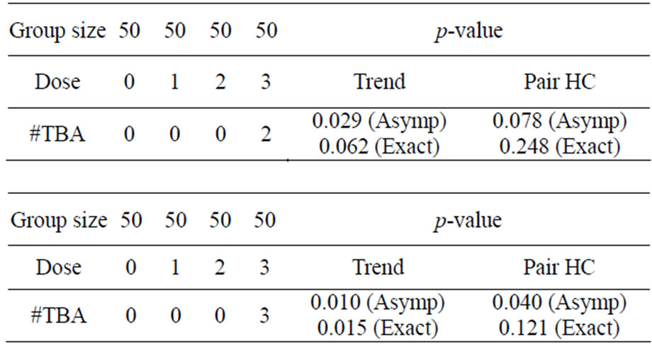
Table 1. Asymptotic and exact p-values showing significant Trend with non-significant pairwise comparisons at α = 0.05.

Table 2. Asymptotic and exact p-values showing non-significant trend with significant pairwise comparison at α = 0.05.
Section 3, we illustrate the application of the two modified pairwise tests on a dataset, and carry out a simulation study in Section 4 to evaluate their power performances. In Section 5, we make some concluding remarks.
2. THEORETICAL DEVELOPMENT
Consider a carcinogenicity study with r + 1 dose groups consisting of one control and r treated groups. Let ni be the number of animals assigned to the ith treatment group, xi be the number of tumor bearing animals observed in the ith treatment group, and di be the dose level for the ith treatment group, with d0 = 0 for control group. Assume that xi has a Binomial distribution as 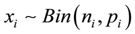 , where pi is the probability of developing tumor by an animal in the ith dose group. The value of pi is generally modeled as
 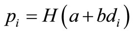 with
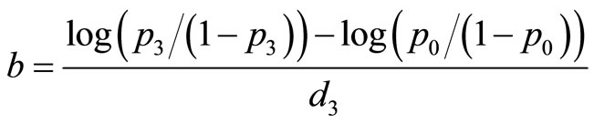
with  , the logistic distribution. The value
  with di = 0 corresponds to the control group. Here, a is a nuisance parameter and b is the parameter of interest.
2.1. Test for Positive Trend
The positive trend is tested by the hypothesis  versus the alternative hypothesis
  , or equivalently by testing
  , vs. H1:pi ≤ pi+1 for all i with strict inequality for at least one i. The value of p* is the overall probability of developing tumor by an animal or overall proportion of tumor bearing animals in the population under null hypothesis. It can be easily shown that the pair
  is jointly sufficient, where
  is the total number of subjects on test in
  groups. The CA test is based on the sufficient statistic.
The CA test for testing the null hypothesis that there is no trend,  versus the alternative hypothesis,
  is given by
N (0, 1), where  and
and .
.
In applications, we replace p* by with
with . The CA test is an asymptotically normal.
The exact test, as derived by Mehta et al., is as follows: Let 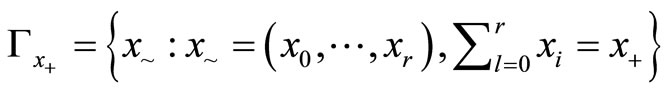 be the sample space which is the collection of all permutations of
  such that
  , the observed total number of tumor bearing animals. Define the critical region for trend test:
 where
where 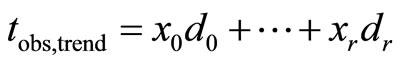 is the realization of the statistic
  , based on the observed data
  . Using the hyper geometric distribution, the probability of each realization of
 .
.
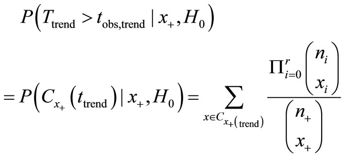
This probability is also known as the table probability, signifying the probability of each table in the all possible permutation of the observed number of tumor bearing animals. The exact p-value for testing H0 (right hand tail) is then
2.2. Pairwise Comparisons
Since the highest dose for a regulatory carcinogenicity study is selected mostly based on the maximum tolerated dose (MTD) criterion, the pairwise comparisons between the high dose group with the control group has special regulatory interest. In this paper we present some results related to pairwise comparisons of high dose group with the control group. The results, however, can be used for the pairwise comparison of any treatment group with control. If we were interested in testing simultaneous multiple contrasts, such as Williams type contrast, the approach described in Hothorn et al. [10] can be used. These methods are based on the quantiles of multivariate normal distribution taking care of the correlation into account as the package MVTNORM.
For pairwise comparison of the highest dose Group r with control with the null hypothesis , and the alternative hypothesis
  , we describe the following two approaches. First note that
 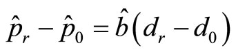 , and
, and
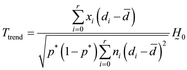
In our first approach, we delete the data from all dose groups except data from dose groups 0 and r, estimate overall proportion of tumor bearing animals as
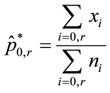 and define the test statistic as
 (1)
(1)
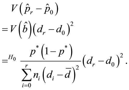
As mentioned, in the derivation of the above test, the variance of  is estimated based on the data from Group r and control only. We will refer to this test as the unconditional test. However, under the null hypothesis of no dose effect, a better estimate of variance of
  can be obtained from the complete data i.e.
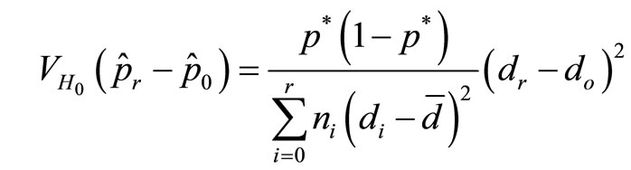 where now p* is estimated as
 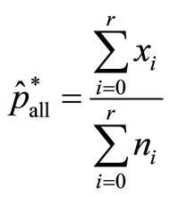 based on data from all dose groups. Using this estimate in the denominator, our second approach is to define the test statistic as
 (2)
(2)
We will refer to this test as the conditional test.
It should be noted that under the linearity assumption of pi with di (the denominator of) the above test is same as the Cochran-Armitage trend test.
2.3. Asymptotic Relative Efficiency of the Conditional and the Unconditional Pairwise Tests
The asymptotic relative efficiency (ARE) of  and
and  is
is

showing that Tpairwise2 is asymptotically more efficient than Tpairwise1.
Hothorn and Bretz [11] proposed (asymptotic) tests for positive trend based on single and multiple contrasts under the assumption of equally spaced dose-levels. For single contrast, test is defined as
 , where
 .
.
For pairwise comparison of Group r and control (r = 0) with c0 = –1 and cr = 1, this test statistic is
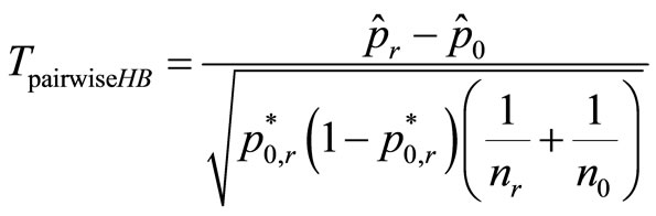 (3)
(3)
The  is estimated by
 , as defined earlier. If the group sizes are equal (i.e. if n0 = n1 = n2 = n3) then it can be shown that the statistics Tpairwise1 and TpairwiseHB are identical.
2.4. Exact Pairwise Test
We now consider the derivation of the exact pairwise tests. Following Mehta et al., the exact p-value for unconditional exact test Texact,pairwise1 based on the data from the Group r and Control, for testing , is calculated as

The exact test for our second approach is as follows. As before, let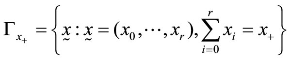 , and define the critical region
 where
where  is the realization of
  based on the observed data
 . The exact p-value for testing
  is calculated as

We will refer to this test as the conditional exact pairwise test.
Proceeding along the lines of Mehta et al., the power of pairwise test is calculated as follows. Let  be such that
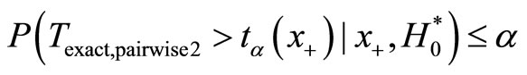 . Then the power of the pairwise test conditional on x+ is
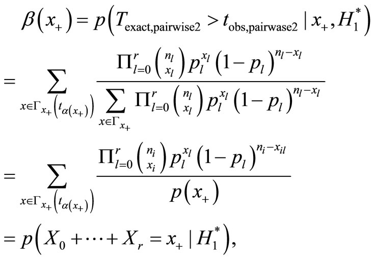
where .
.
The above power can be evaluated for exact test using the hyper geometric distribution and appropriate critical regions under conditional and unconditional situations.
We compare the relative power of three asymptotic pairwise tests, as well as that of the two exact tests TExact, pairwise1 and TExact, pairwise2. For evaluation of their power functions, we performed simulations and calculated the percentage of times the null hypothesis was rejected when the alternative hypothesis was true. The SAS proc Stratify and SAS proc Multtest [12] are very convenient for the calculation of these exact probabilities.
3. EXAMPLE
Consider a carcinogenicity study with four treatment groups namely, control, low, medium, and high dose groups each with 50 animals, and dose scores 0, 1, 2, and 3, respectively. Suppose we observe a total of 10 animals developed a certain tumor type with 0, 2, 3 and 5 tumor bearing animals in control, low, medium, and high dose groups, respectively. We would like to perform a pairwise comparison of the high dose group with the control. The null hypothesis  against alternative
 . The results using the normal approximation test are Tpairwise1 = 2.294, Tpairwise2 = 2.418, and TpairwiseHB = 2.294 with corresponding p-values as 0.0109, 0.0078, and 0.0109, respectively.
For exact test we have tobs,pairwise1 = tobs,pairwise2 = x0d0 + x3d3 = 15. Table 3, given below, shows all possible values of Tpairwise1 along with their table probabilities and the right tail probabilities for pairwise comparison of high dose with control calculated from data after dropping low and medium dose groups using SAS proc Stratify.
Table 4 given below shows all possible values of Tpairwise2 along with their table probabilities and the right tail probabilities for pairwise comparison of high dose with control calculated from all data using the scores 0, 0, 0 and 3 in SAS proc Multtest.
The results from Tables 3 and 4 show that both the tableand right-tail probabilities for the two pairwise exact

Table 3. Pair comparison of control with high dose group after deleting the low and medium dose groups.
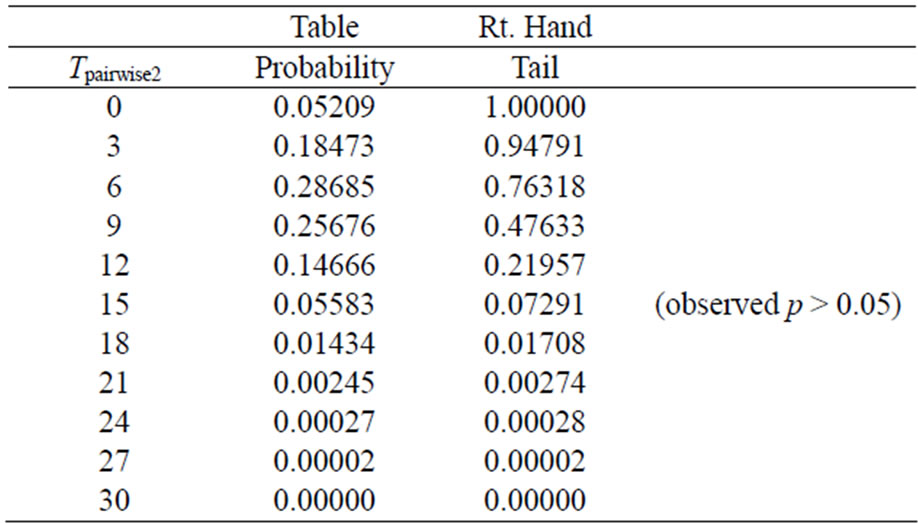
Table 4. Pairwise comparison of high dose with control using all data.
tests may go in either direction. For example for the observed number of 0, 2, 3 and 5 tumor bearing animals, we have tobs,pairwise1 = tobs,pairwise2 = x0d0 + x3d3 = 15, and the p-value after deleting the low and medium dose groups is ppairwise1 = 0.0281, and that using data from all dose groups is ppairwise2 = 0.0729 i.e. the p-value after deleting the low and medium dose groups is smaller than the p-value using data from all dose groups. On the other hand if the observes number of tumor bearing animals were 2, 2, 3, and 3, then tobs,pairwise1 = tobs,pairwise2 = x0d0 + x3d3 = 9. The p-value after deleting the low and medium dose groups would be ppairwise1 = 0.5, and that using data from all dose groups would be ppairwise2 = 0.4763. In this case the p-value for pairwise exact test after deleting the low and medium dose groups would be larger than the p-value for the pairwise exact test using the data from all dose groups.
4. SIMULATION STUDY OF POWER CALCULATION
Consider a carcinogenicity study with four treatment groups namely, control, low, medium, and high dose groups each with 50 animals, and dose scores 0, 1, 2, and 3, respectively. The power was calculated for different choices background incidence rate in the control group (p0). The incidence rate for the high dose group (p3) was then chosen by a certain increment (δ) over p0. The incidence rate for the low dose group (p1) and that for medium dose group (p2) were calculated using a logistic model as follows:
If 
and
 then
then
 and
and with di = i and i = 0, 1, 2, and 3. The values of the power were calculated by finding the percentages of times the null hypothesis was rejected when the alternative was true in a simulation with 1000 loops. Table 5 shows the calculated power using the asymptotic normal approximation and Figure 1 gives the graphical representation of the results.
Table 6 shows the calculated power using the exact test and Figure 2 gives the graphical representation of the results.
The simulation results show that asymptotic normal test Tpairwise2 is always a more powerful compared to Tpairwise1 or TpairwiseHB. The two tests Tpairwise1 and TpairwiseHB have similar power (as sample sizes are taken to be same). The pairwise exact test using data from all dose groups has more power compared to test based on data deleting the two middle dose groups for small values of p0 and δ.
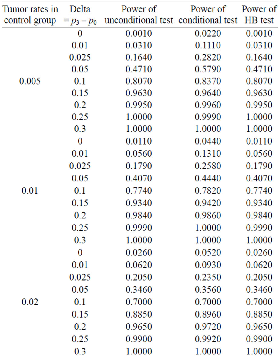

Table 5. Power calculated using the normal approximation for unconditional, conditional, and Hothorn Bretz tests.
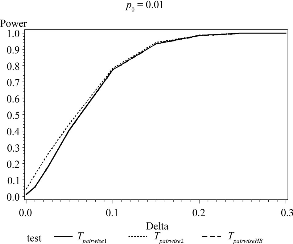

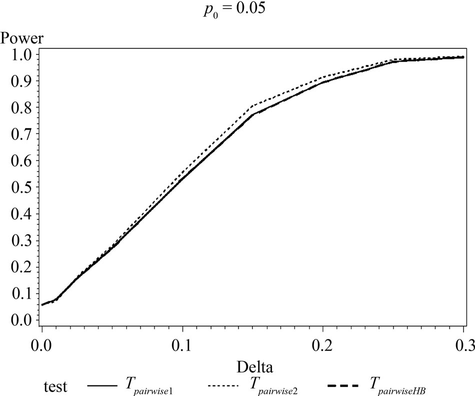

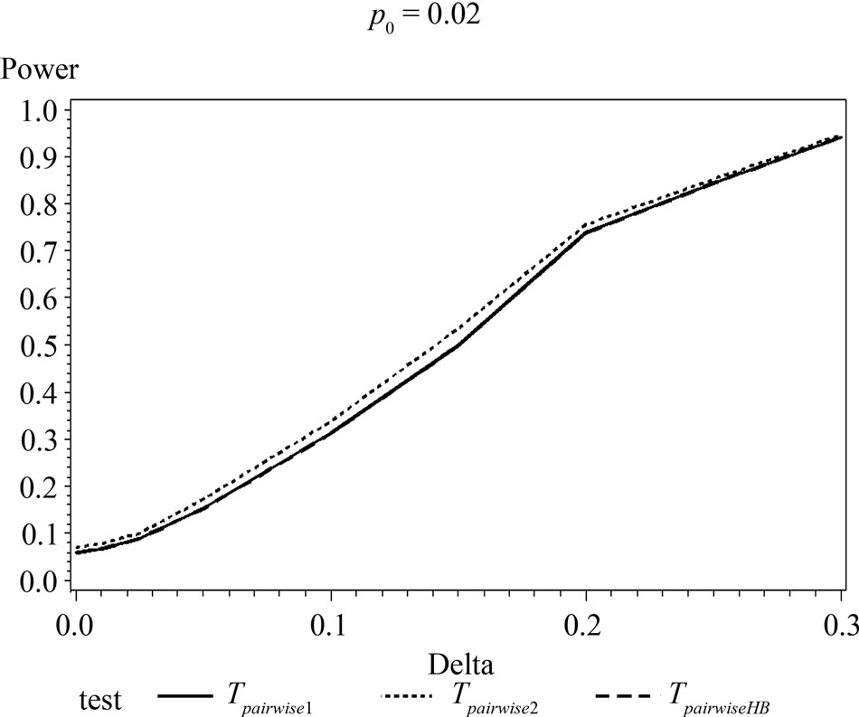
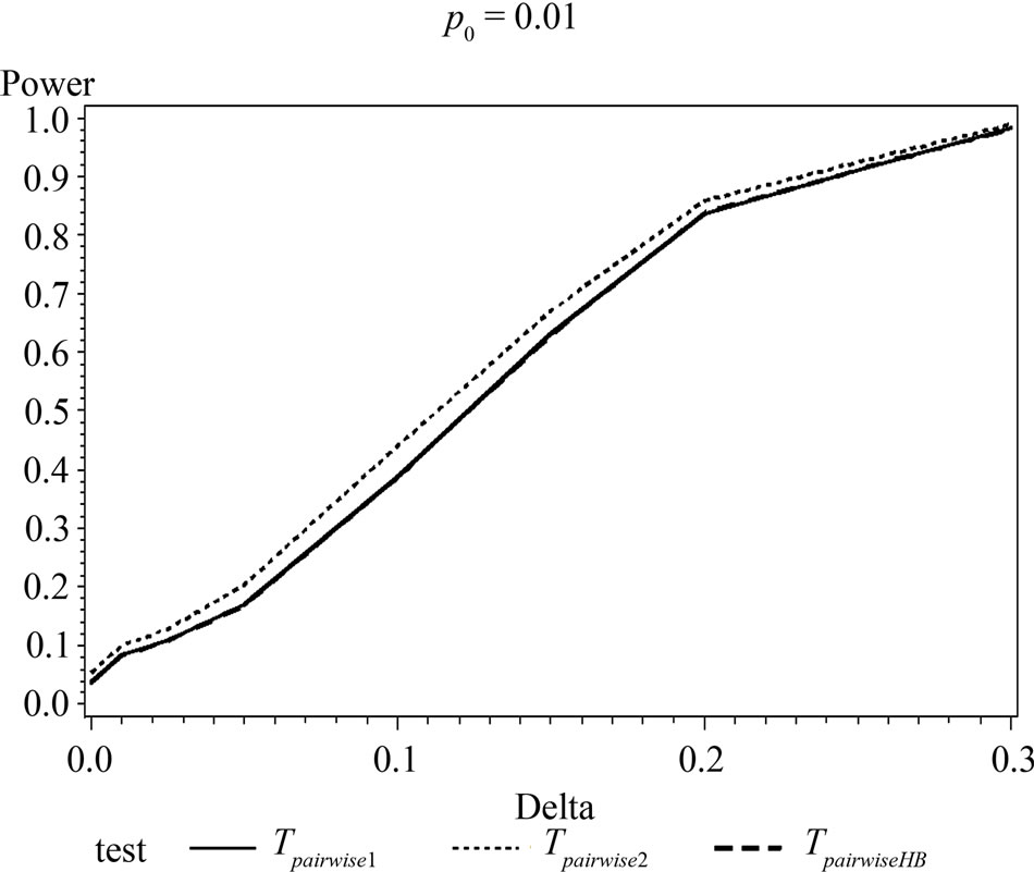
Figure 1. Graphical representation of power vs. delta for given p0 using normal approximation for pairwise comparison of control and high dose group. (Where ---------: power of unconditional test and ………: power of conditional test.)
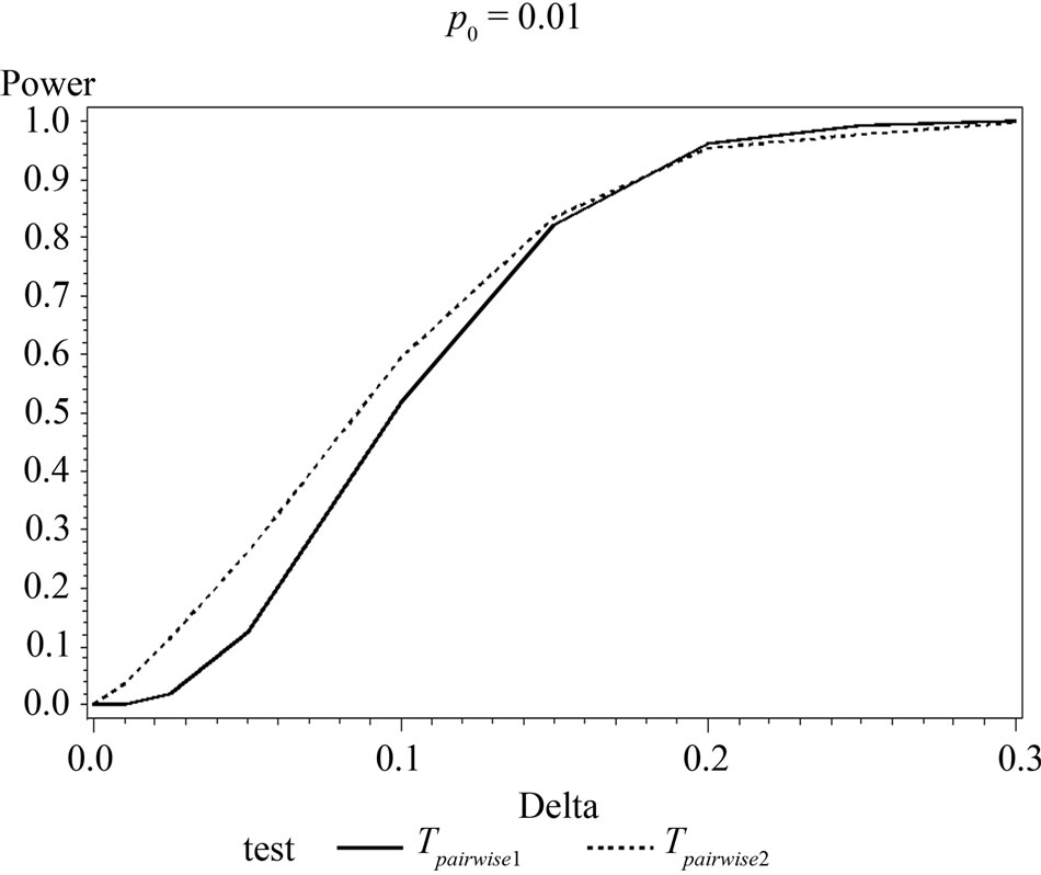
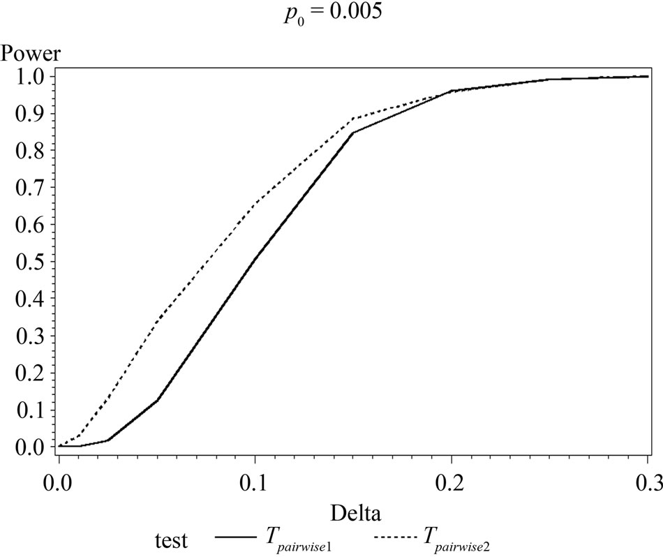

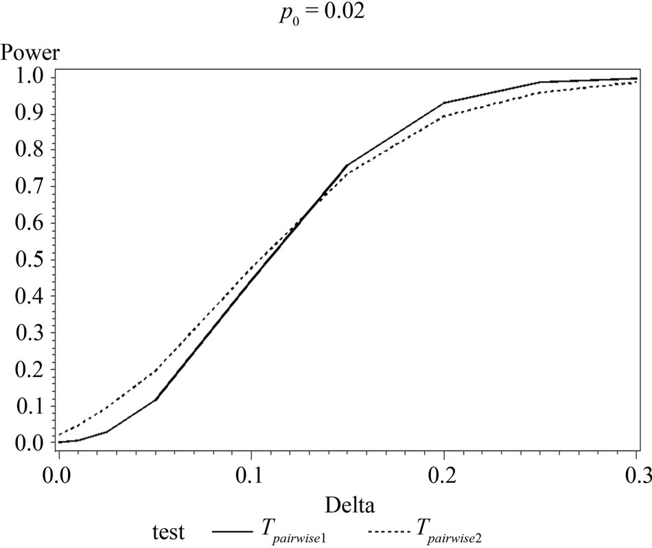
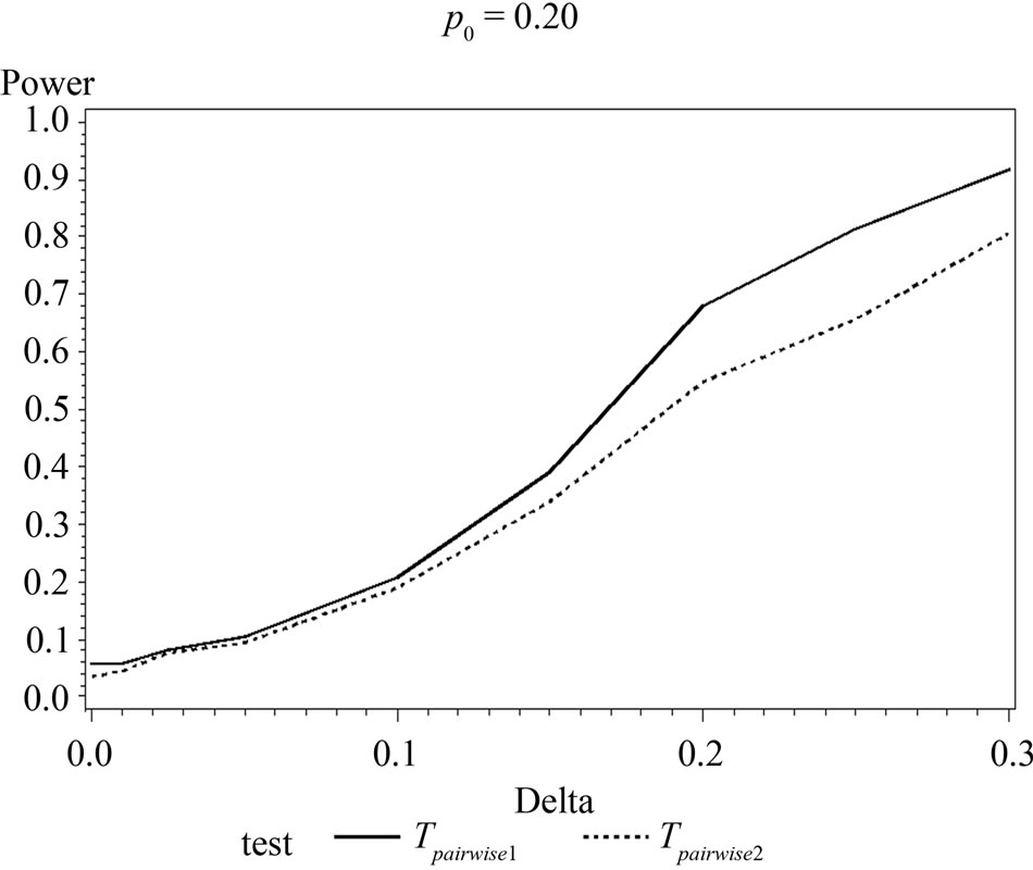
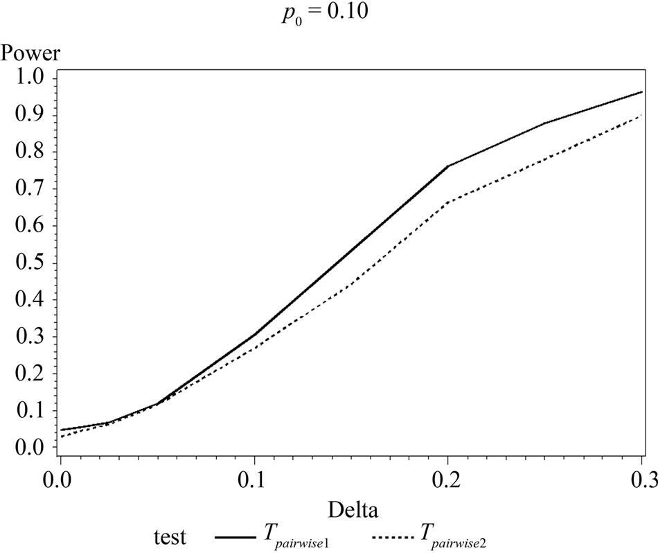
Figure 2. Graphical representation of power vs. delta for given p0 using exact test for pairwise comparison of control and high dose group. (where ---------: Power of unconditional test and ………….: Power of conditional test.)

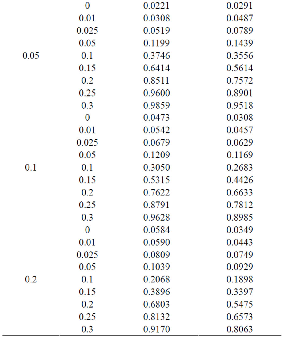
Table 6. Power calculated using the exact test for unconditional and conditional tests.
When p0 and/or δ become (s) large the pairwise exact test that deletes the data from two middle dose groups showed better power.
5. CONCLUSIONS
In this paper, we discussed the topic of pairwise comparison of the high dose group with control in a typical carcinogenicity study. We proposed two tests procedure, one based on data only from the two dose groups to be compared and one based on data from all dose groups. We elaborated both exact and normal approximation version of our proposed tests.
Through a simulation, we compared the power performances of these tests. For the comparison of high dose group with control group in a typical four dose group carcinogenicity study, the simulation results showed that the power of the asymptotic normal test using data from all dose groups is asymptotically more efficient and hence is always more powerful than that of the test using data from high and control groups only. For exact test, neither of the two tests showed uniformly better power than the other. The pairwise exact test using data from all dose groups showed more power than that of the test based on data deleting the two middle dose groups for tumor types with low background rate and/or drug with small carcinogenic effect, while the pairwise exact test using data from all dose groups showed less power than that of the test based on data deleting the two middle dose groups for tumor types with high background rate and/or drug with large carcinogenic effect. However, since a test that drops part of the data is asymptotically less efficient, we recommend that for the pairwise comparison one uses tests that use the data from all dose groups.
6. ACKNOWLEDGEMENTS
The authors are deeply indebted to Drs. Stella G. Machado and Karl K. Lin, Division of Biometrics-6, US Food and Drug Administration, for their helpful advices and comments to improve and complete this work.
REFERENCES
- Cochran, W.G. (1954) Some methods of strengthening the common χ2 tests. Biometrics, 10, 417-451. Hdoi:10.2307/3001616
- Armitage, P. (1955) Tests for linear trend in proportions and frequencies. Biometrics, 11, 375-386. Hdoi:10.2307/3001775
- Tarone, R.E. (1975) Test for trend in life table analysis. Biometrika, 62, 679-690. Hdoi:10.1093/biomet/62.3.679
- Tarone, R.E. (1982) The use of historical control information in testing for a trend in Poisson means. Biometrics, 38, 457-462. Hdoi:10.2307/2530459
- Hoel, D.G. and Yanagawa, T. (1986) Incorporating historical controls in testing for a trend in proportions. Journal of the American Statistical Association, 81, 1095-1099. Hdoi:10.1080/01621459.1986.10478379
- Tamura, R.N. and Young, S.S. (1986) The incorporation of historical control information in tests and proportions: Simulation study of Tarone’s Procedure. Biometrics, 42, 343-349. Hdoi:10.2307/2531054
- Peto, R., Pike, M.C., Day, N.E., Gray, R.G.K, Lee, P.N. Parish, S., Peto, J., Richards, S. and Wahrendorf, J. (1980) Guidelines for sample sensitive significance test for carcinogenic effects in long-term animal experiments. IARC Monographs on the Evaluation of the Carcinogenic Risk of Chemicals to Humans, Suppl. 2, Long-Term and ShortTerm Screening Assays for Carcinogens: A Critical Appraisal, IARC, Lyon, 311-426.
- Bailer, A.J. and Portier, C.J. (1988) Effects of treatmentinduced mortality and tumor-induced mortality on tests for carcinogenicity in small samples. Biometrics, 44, 417-431. Hdoi:10.2307/2531856
- Mehta, C.R. and Patel, N.R. and Senchaudhuri, P. (1998) Exact power and sample-size computations for the Cochran-Armitage trend test. Biometrics, 54, 1615-1621. Hdoi:10.2307/2533685
- Hothorn, L.A., Sill, M. and Schaarschmidt, F. (2010) Evaluation of incidence rates in pre-clinical studies using a Williams-type procedure. The International Journal of Biostatistics, 6, 1557-4679. Hdoi:10.2202/1557-4679.1180
- Hothorn, L.A. and Bretz, F. (2000) Evaluation of animal carcinogenicity studies: Cochran-armitage trend test vs. multiple contrast tests. Biometrical Journal, 42, 553-567. Hdoi:10.1002/1521-4036(200009)42:5<553::AID-BIMJ553>3.0.CO;2-R
- SAS Institute Inc., (2009) Multtest procedure. SAS user’s guide 9.2. 2nd Edition, SAS Institute Inc., Cary, 4176-4242.
NOTES
*Disclaimer: This article reflects the views of the authors and should not be construed to represent FDA’s views or policies.